In this post, we are going to do a nonlinear buckling analysis for a thin arch shell under uniformly distributed pressure. The configuration of the arch shell is as follows

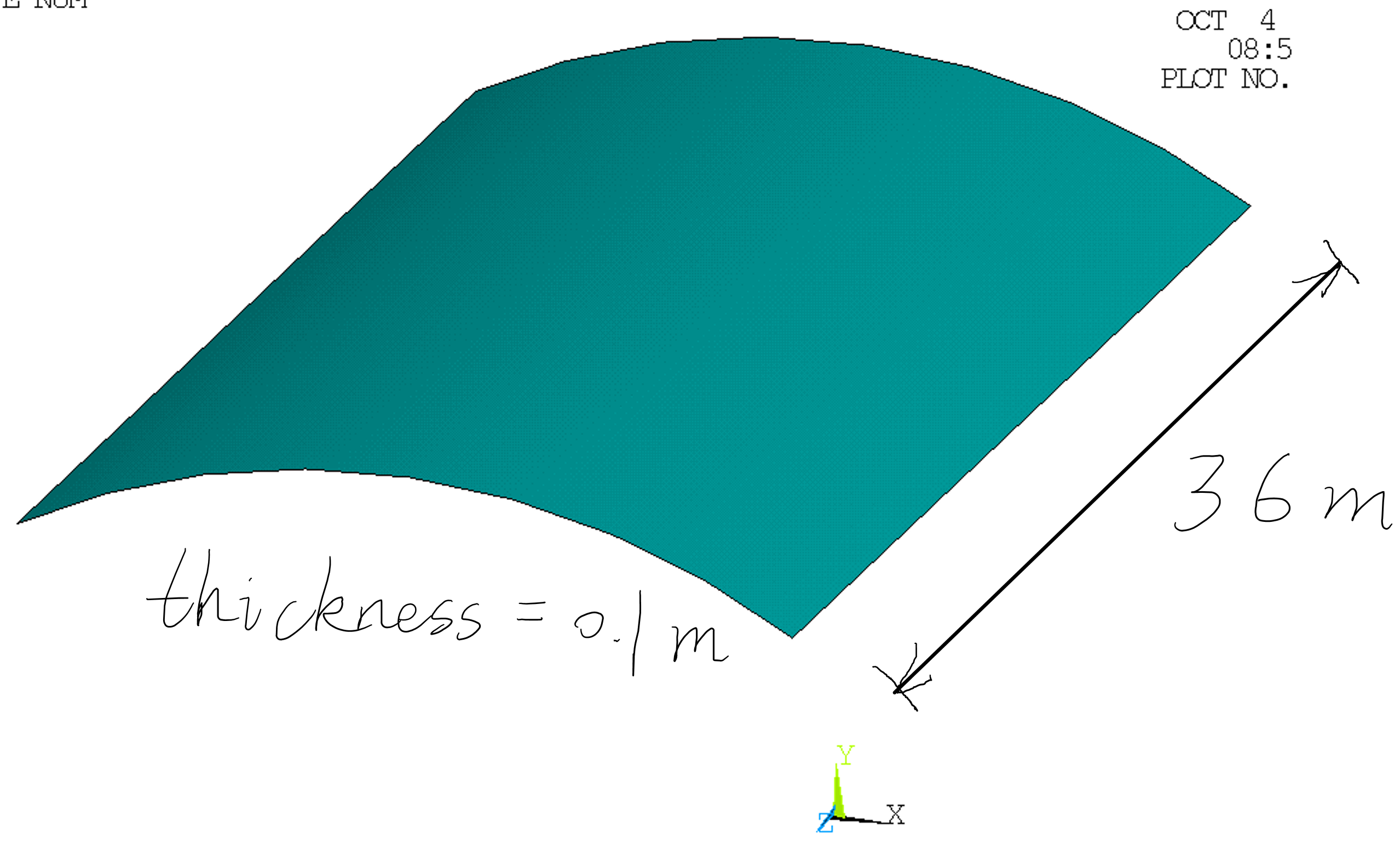
During the analysis, a linear buckling analysis will be conducted first to obtain the 1st-order eigenvalue (i.e. the linear buckling load) and eigenmode (i.e. buckling mode). Then a nonlinear buckling analysis will be done by: 1. modifying the material model to include material nonlinearity; 2. updating the geometry to introduce initial imperfections; 3. scaling up the pressure to about 120% of the linear buckling load. 

When modifying the material model, the bilinear isotropic hardening (BISO) material model is used. The geometry is updated using UPGEOM and 5% of the 1st-order buckling mode is superimposed on the initial geometry as imperfections. After scaling up the pressure, it is possible that the solution will not converge in the end. So plotting the load-deformation curve (i.e. equilibrium path) is very useful to estimate the limit load.

The APDL for the linear buckling analysis is as follows (annotations are in lowercase)

FINISH
/CLEAR
/FILNAME,BUCKLING
/TITLE,BUCKLING ANALYSIS
/PREP7
ET,1,SHELL181
MP,EX,1,2E11
MP,PRXY,1,0.2
MP,DENS,1,7800
SECTYPE,1,SHELL
SECDATA,0.1,1,0.0,5
SECOFFSET,MID
CSYS,1				!Cylindrical with global Cartesian Z as the axis of rotation
K,,20,60,0
K,,20,60,36
K,,20,120,36
K,,20,120,0
A,1,2,3,4
/VIEW,1,1,2,3
/REPLOT
AATT,1,,1,,1
AESIZE,ALL,2
MSHAPE,0,2D
MSHKEY,1
AMESH,ALL
EPLOT
CSYS,0
NSEL,S,LOC,X,-10.1,-9.9
NSEL,A,LOC,X,9.9,10.1
D,ALL,UX,,,,,UY,UZ
ALLSEL
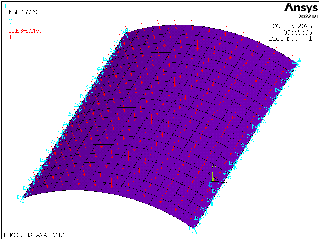
SFE,ALL,1,PRES,,1                  !apply unit pressure
/PSF,PRES,NORM,2,0,1
/REPLOT
FINISH
/SOLU
ANTYPE,STATIC
PSTRES,ON
SOLVE
FINISH
/SOLU
ANTYPE,BUCKLE
BUCOPT,LANB,6,0,0
MXPAND,6,0,0,1
SOLVE
FINISH
/POST1
SET,FIRST
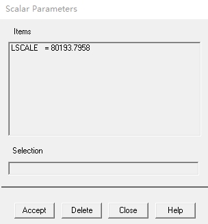
*GET,LSCALE,ACTIVE,,SET,FREQ       !get buckling load
PLDISP,0                           !plot buckling mode
SET,NEXT
PLDISP,0
SET,NEXT
PLDISP,0
SET,NEXT
PLDISP,0
SET,NEXT
PLDISP,0
SET,NEXT
PLDISP,0
FINISH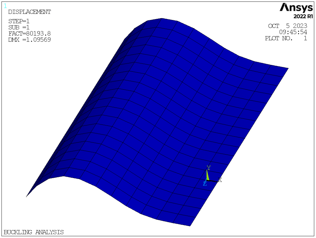

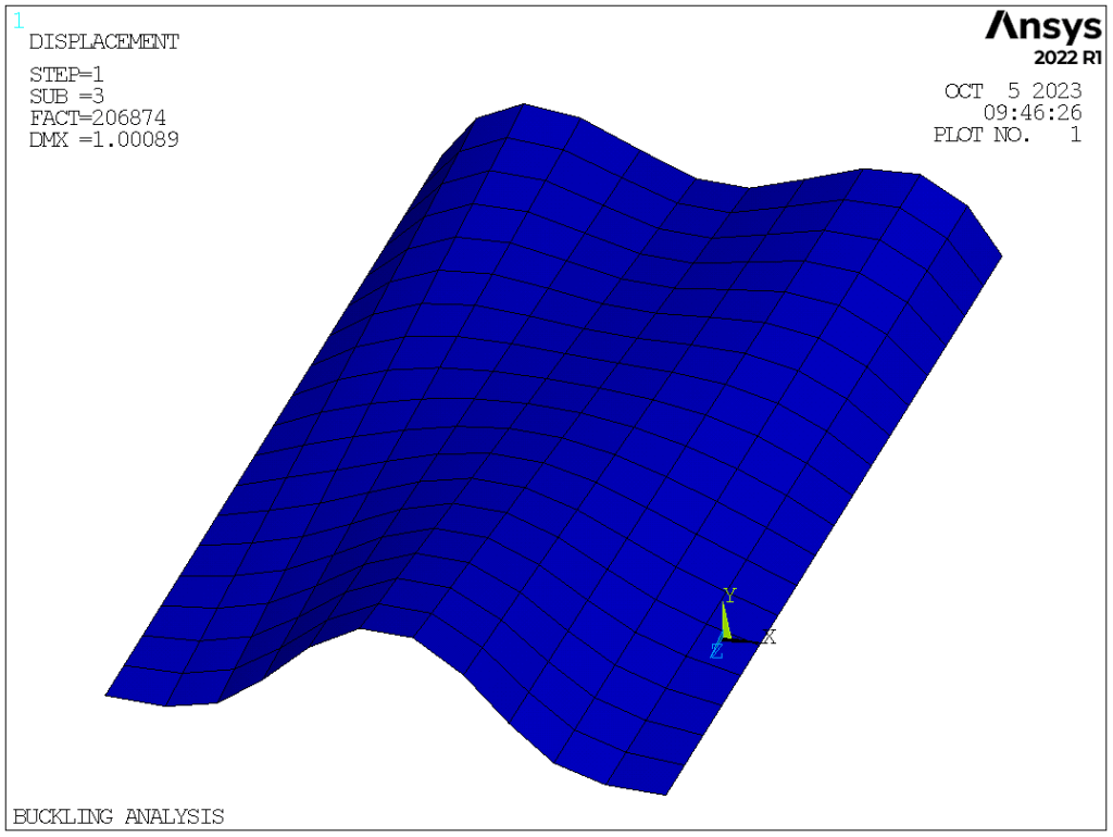
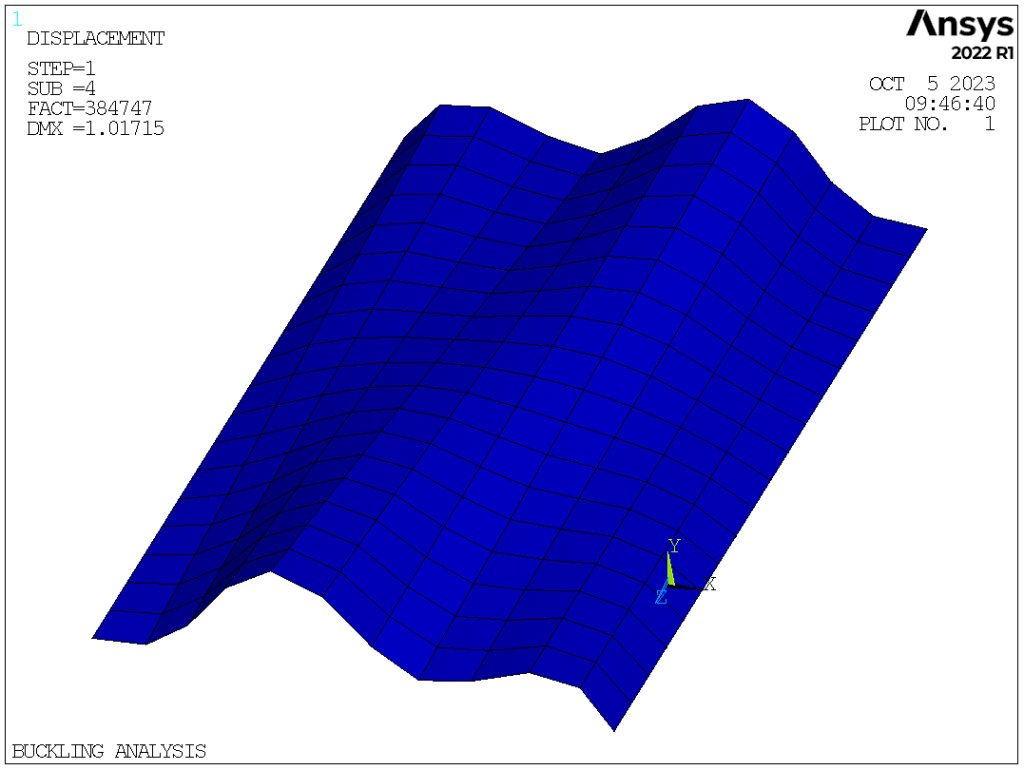
The buckling load and the first five buckling modes.

The APDL for the ensuing nonlinear buckling analysis is as follows (annotations are in lowercase)

/PREP7
TB,BISO,1,1,2	!Bilinear Isotropic Hardening Model: Yield stress & Plastic tangent modulus
TBDATA,,2E8,0
! TBPLOT,BISO,1
! TBLIST,BISO,1
UPGEOM,0.05,1,1,'BUCKLING','rst'!Adds displacements from a previous analysis 
			!and updates the geometry of the finite element model 
			!to the deformed configuration.
DSYS,1		!Activates a display coordinate system for geometry listings and plots.
/VIEW,1,,,-1
/REPLOT
DSYS,0
FINISH
/SOLU
ANTYPE,STATIC
SFSCALE,PRES,1.2*LSCALE		!scales surface loads on elements: 120%
TIME,1.2*LSCALE		!Time at the end of the load step (use time as load indicator)
NLGEOM,1
OUTRES,ALL,ALL
LNSRCH,ON		!Activates a line search to be used with Newton-Raphson.
NSUBST,200,,,1
SOLVE
FINISH
/POST26
CSYS,1			!switch to cylindrical coordinate system
N1=NODE(20,90,18)       !get the node number of the node in the middle
NSOL,2,N1,U,X,DEFLECTION
/AXLAB,X,MIDNODE DISPLACEMENT (m)
/AXLAB,Y,PRESSURE (Pa)
/GROPT,REVX,1		!Plots the values on the X-axis in reverse order.
XVAR,2
PLVAR,1
FINISH
/POST1
SET,LIST
SET,1,21
PLDISP,1
PLNSOL,U,X
PLNSOL,S,1
PLNSOL,S,EQV
PLNSOL,EPPL,EQV
FINISH

BISO material model

Observing initial imperfections by changing the display coordinate system

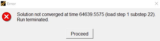
Convergence error (click proceed)

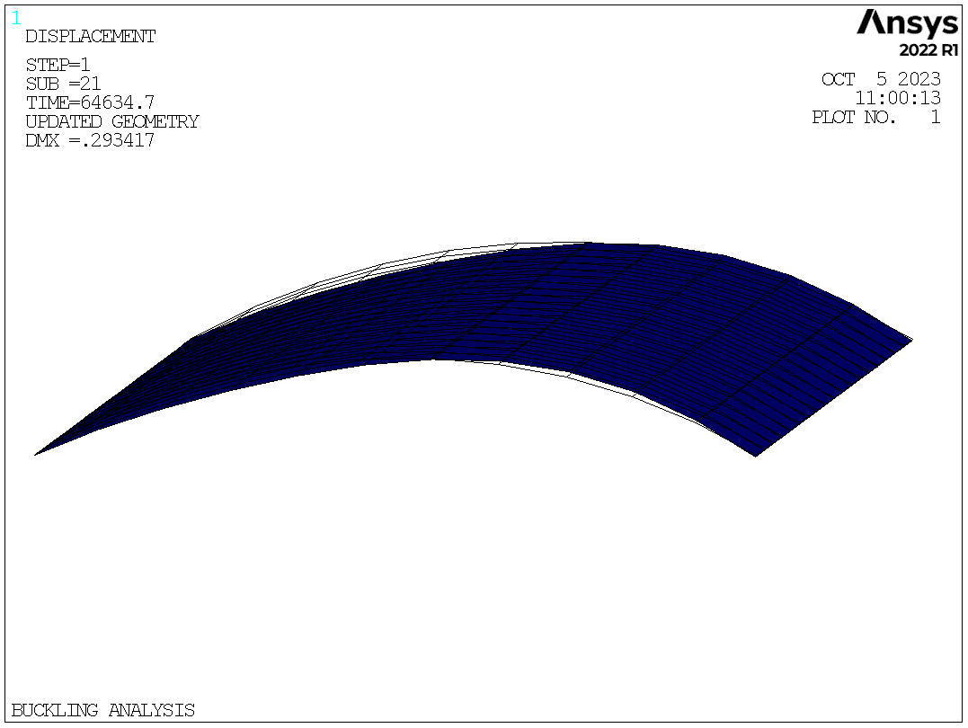
Select the penultimate load step and plot the deformation

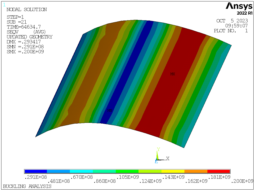
The equivalent stress

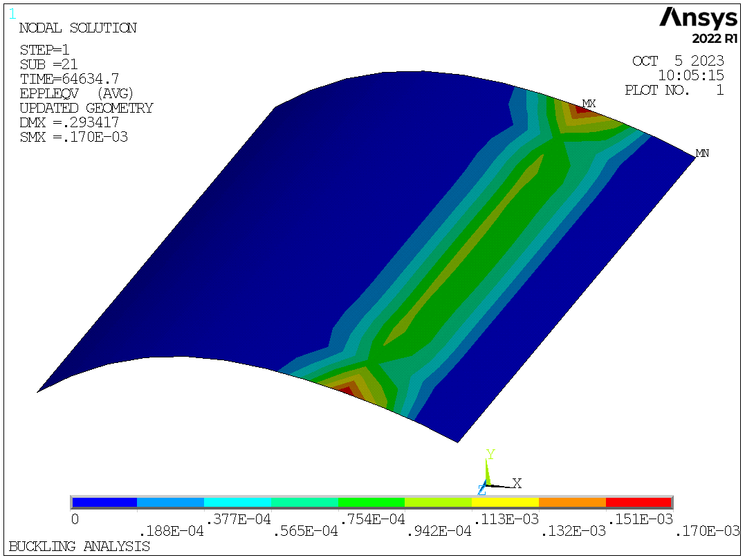
The equivalent plastic strain

The equilibrium path

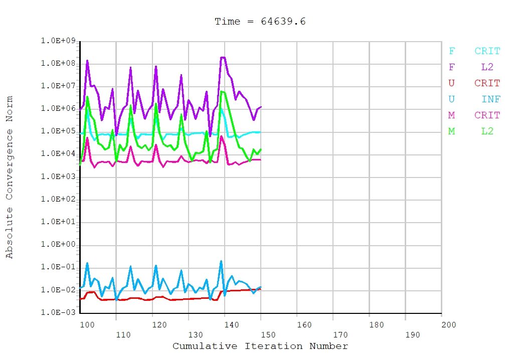
From the equilibrium path, the ultimate pressure is between 60000Pa and 70000Pa, which is below the 1st-order buckling load 80193.7958Pa. By checking the penultimate load step, we can know the calculated ultimate pressure is 64635Pa (load step 1 substep 21). The maximum deformation of the shell is about 0.29m. The maximum stress has approached to yield strength. The region with large equivalent stress coincides with the region with high equivalent plastic strain. 

We can also calculate post-buckling behavior and capture the descending segment of the equilibrium path. The arc-length method should be used and it is a good practice to control the termination of the solution using ARCTRM. For example, we can terminate the solution when the displacement of the mid node along X direction exceeds 0.15m. 

The APDL for post-buckling analysis using the arc-length method is as follows (annotations are in lowercase)

/PREP7
TB,BISO,1,1,2	!Bilinear Isotropic Hardening Model: Yield stress & Plastic tangent modulus
TBDATA,,2E8,0
! TBPLOT,BISO,1
! TBLIST,BISO,1
UPGEOM,0.05,1,1,'BUCKLING','rst'!Adds displacements from a previous analysis 
			!and updates the geometry of the finite element model 
			!to the deformed configuration.
FINISH
!use arch-length method:
/SOLU
ANTYPE,STATIC
SFSCALE,PRES,1.2*LSCALE
TIME,1.2*LSCALE
NLGEOM,ON
OUTRES,ALL,ALL
CSYS,1
NN=NODE(20,90,18)
CSYS,0
ARCLEN,ON
ARCTRM,U,0.15,NN,UX !Controls termination of the solution when the arc-length method is used.
NSUBST,200
SOLVE
FINISH
/POST26
CSYS,1		!switch to cylindrical coordinate system
N1=NODE(20,90,18)
NSOL,2,N1,U,X,DEFLECTION
/AXLAB,X,DISPLACEMENT (m)
/AXLAB,Y,PRESSURE (Pa)
/GROPT,REVX,1	!Plots the values on the X-axis in reverse order.
XVAR,2
PLVAR,1
FINISH										
/POST1
SET,LIST
SET,LAST
PLNSOL,U,X
PLNSOL,S,EQV
PLNSOL,EPPL,EQV
FINISH

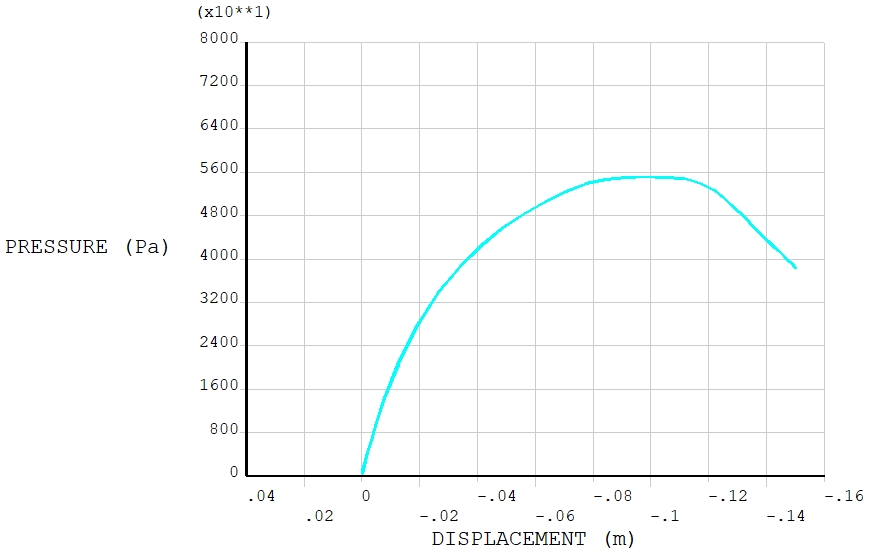
The equilibrium path using the arc-length method

The load steps (Maximum pressure=64488Pa)

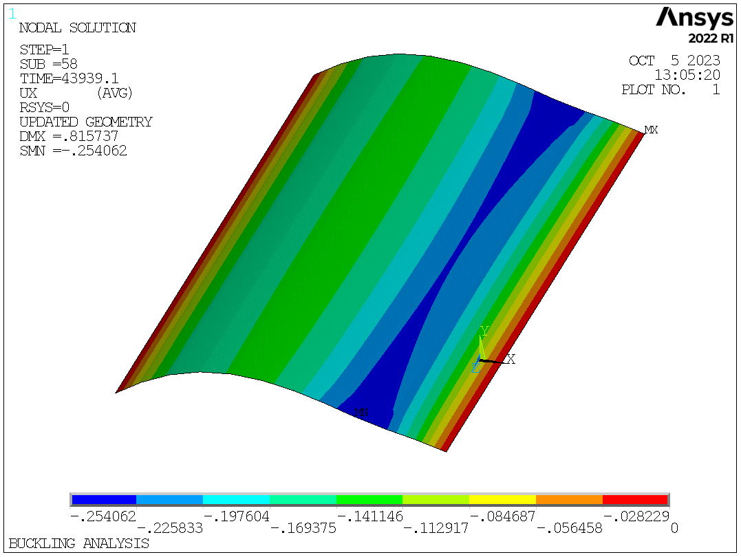
Displacement in X direction when the solution stops

Using the arc-length method, the descending section of the equilibrium path shows the response after buckling. The maximum pressure is 64488Pa, which is close to the previous calculation using the line search method. When Ux at the mid node exceeds 0.15m, the maximum Ux is about 0.25m happening on the right side.

It is also possible to consider larger imperfections, for example, consider 10% of the 1st-order buckling mode: UPGEOM,0.1,1,1,’BUCKLING’,’rst’

The maximum pressure (55142Pa) decreases as the extent of imperfection increases.