A rotating reference frame is usually used when modelling the flow through a table fan, a blower fan, an impeller, or a ceiling fan as shown in Figure 1. SolidWorks Flow Simulation allows for the use of rotating reference frames within the computational domain. These rotating reference frames can be defined either globally or locally.

Figure 1. A ceiling fan.

If defined globally, the model assumes that all of the walls rotate at the same speed of the reference frame and that the corresponding Coriolis and centrifugal forces are taken into account.

When defined locally, the rotating region is only applied to that area (i.e. area around a fan or impeller). The region must be defined as a component in the model to be defined as rotating. Two solution approaches are available:

• In the Averaging approach, the fluid flow within the rotating region is calculated in the rotating region’s local reference frame. Flow field parameters are transferred from adjacent flow regions to the rotating region’s boundary conditions. The flow field must be axially symmetric at the rotating region’s boundary. The rotating regions must not intersect with each other.
• In the Sliding Mesh approach, it is assumed that the flow field is unsteady and it is available for transient analysis only. This assumption allows for obtaining more accurate simulation when the rotor-stator interaction is strong. However, because this approach requires an unsteady numerical solution, it is computationally more demanding than the Averaging

In this example we will use the Averaging approach to analyse the ceiling fan. The fan is located in a large space, and only part of the space is modelled in this simulation (see Figure 2), thus the side walls are not present. The four sides of the computational domain are positioned reasonably far from the fan, and assigned environmental boundary conditions. The fan rotates with a speed of 31.4 rad/s.

Figure 2. The space and the boundary conditions on four sides.

When defining the analysis type using the wizard, choose Internal because the entire fan is surrounded by the space. Also, check Rotation and choose Local region(s) (Averaging) as shown in Figure 3.

Figure 3. Analysis type.

To define the rotation region, a virtual part has been created in the environment of the assembly as shown in Figure 4. Also be sure to exclude the virtual part in Component Control after it is specified as rotating, otherwise an error will occur when solving the model.

Figure 4. Creating a component in the model to define the rotating region.

Notice that the rotating region used in this simulation does not include the full length of the hanging rod of the fan. While a rotating region could include the full length, an alternative approach is to define a Real Wall boundary condition when there is an entire wall moving in the tangential direction with respect to the fluid, as shown in Figure 5.

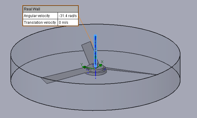
Figure 5. Real wall boundary condition.

Right-click Input data in the Flow Simulation analysis tree and select Calculation Control Options, check Iterations and set it to 3600, as shown in Figure 6.

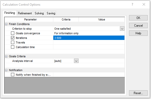
Figure 6. Calculation control options.

After solving the model, a flow velocity cut plot is shown in Figure 7. Figure 8 and Figure 9 display the pressure surface plot on the bottom side and top side of the blades, respectively. The pressure is lower as the air enters the fan from the top side, and it increases as the air exits the fan from the bottom side. The difference between the static pressure at the fan exit and entrance is referred to as pressure drop.

Figure 7. Flow velocity cut plot.

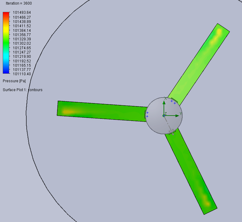
Figure 8. Surface pressure on the bottom side.

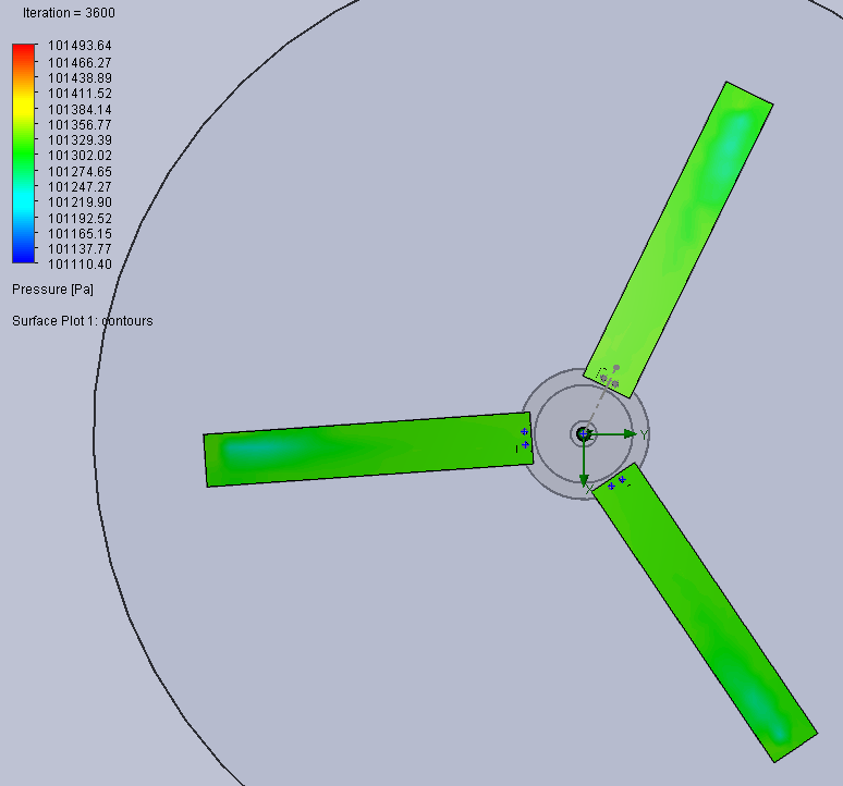
Figure 9. Surface pressure on the top side.

A sketch is created at a plane 100mm beneath the ceiling (see Figure 10). Using the sketch as reference, flow trajectories can be defined as shown in Figure 11.

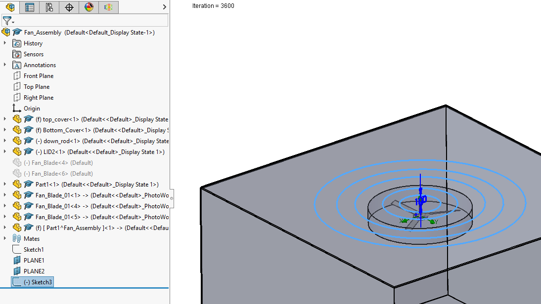
Figure 10. Creating a sketch for flow trajectories.

Figure 11. Flow trajectories.