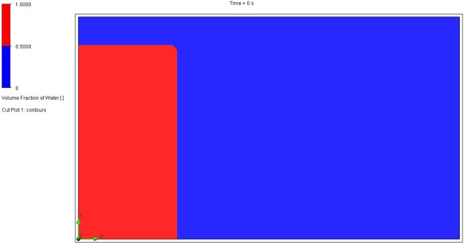
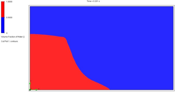
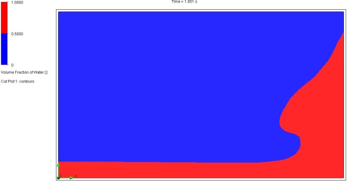
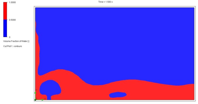
In this post, we are going to use the free surface option to solve for a dam-break problem. The body of water is initially contained in a region on the left side. Then the water is released suddenly and starts to flow into the empty regions of the tank. Water is free to spill from the top of the tank. The following slide show illustrates the water flow in the first 1.5 seconds, with blue regions indicating air and red regions indicating water.

What does ‘free surface’ mean?

Free surface represents a type of analysis where two immiscible fluids are modelled. When two fluids are immiscible, they are completely insoluble in each other. A free surface is an interface between immiscible fluids, for example, a liquid and a gas. In this problem, we are considering the free surface between water and air.

Note:

Any phase transitions (including humidity, condensation, cavitation), rotation, surface tension and boundary layer on an interface between immiscible fluids are now allowed. In simpler terms, the simulation will treat the fluids as if they don’t change state, don’t swirl around, and don’t have special surface effects at their boundaries. This simplification can make the simulation easier to run and understand, but it might not be accurate for situations where these phenomena are important. For example, a simulation of boiling water would need to account for phase transitions, while a simulation of water flowing through a pipe might need to consider surface tension and boundary layers.

General steps:

The geometric model of this problem is shown below. Since a 2D computational domain will be used, two solid bodies with limited depth have been created, with one representing the water domain and the other representing the tank.

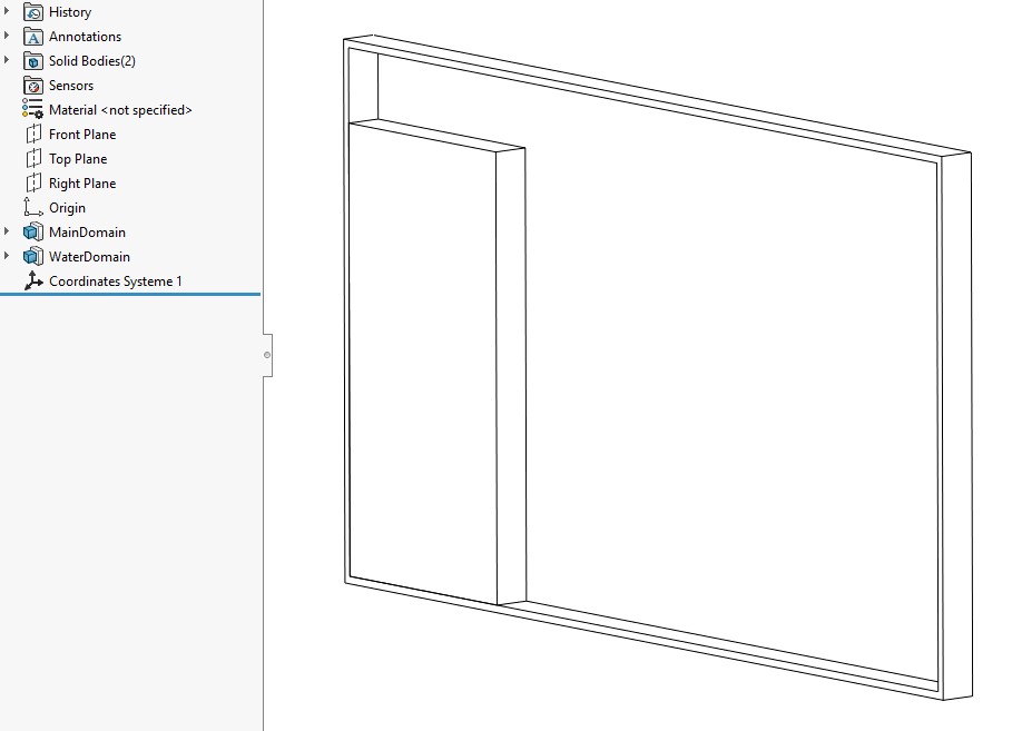
Figure 1. 3D model.

Figure 2 shows the settings for analysis type. For a quick demo, we will simulate the first 1.5s (time-dependent), with gravity and free surface options checked.

Figure 2. Analysis type.

For the default fluid, make sure air and water are selected. Automatically, the ‘Default fluid type’ should be set to ‘Immiscible Mixture’, as shown in Figure 3.

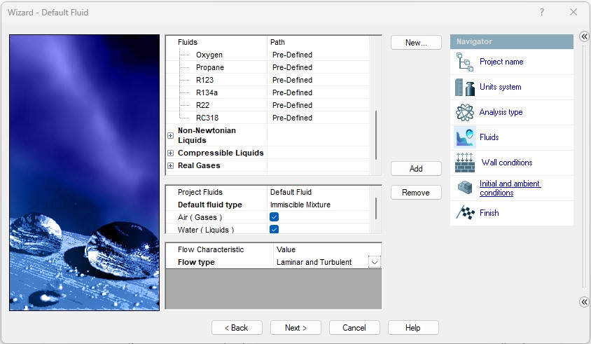
Figure 3. Default fluid.

For the initial conditions, the turbulence intensity is increased from the default 0.05% to 2% to yield more realistic wave front behaviour and splash/overturn behaviour.

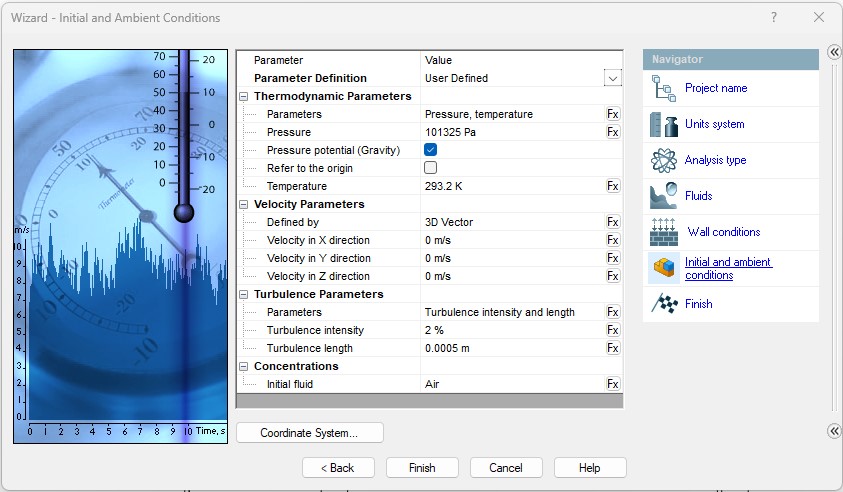
Figure 4. Initial and ambient conditions.

Figure 5 shows the computational domain settings. The computational domain is slightly larger than the inner space of the tank.

Figure 5. Computational domain.

As water is free to spill over the tank from above, the top of the tank is set to pressure opening – environmental pressure. Under ‘Substance Concentrations’, the initial fluid distribution is specified as ‘Air’, which is a constant distribution (see Figure 6).

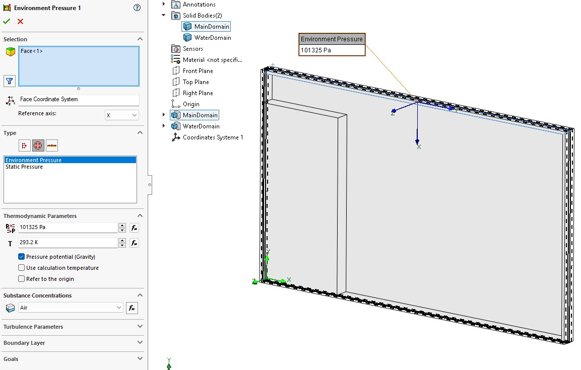
Figure 6. Boundary condition.

For initial conditions, select the solid body representing the water domain and make sure to ‘Disable solid components’. Under ‘Substance Concentrations’, the initial fluid distribution is specified as ‘Water’, which is also a constant distribution (see Figure 7).

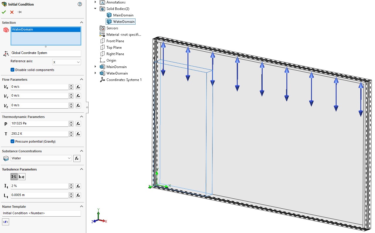
Figure 7. Initial condition.

For a quick trial calculation, a manual coarse mesh has been generated as shown in Figure 8. The results in the above slide show are obtained using this coarse mesh in less than a minute. The mesh can be refined further for more accurate results.

Figure 8. An initial coarse mesh.