This post originates from a project validating the drop test experiment (see Figure 1) in a case study—Analytical and Experimental Study on Drop Test of Electronic Devices (Lamar University, 2021)—using Transient Structural analysis in ANSYS.

Figure 1. The drop test set-up.

There are several important questions to ask before the simulation:

 

For this drop test simulation, should I use Transient Structural analysis or Explicit Dynamics?

The general rule of thumb is, Transient Structural analysis is efficient and accurate for elastic or moderate impacts, and Explicit Dynamics is suitable for high-speed, nonlinear, or destructive impacts. Both approaches are valid, and the right choice depends on the physics you need to capture and the level of computational effort you can afford.

 

When using Transient Structural analysis to simulate a drop test in ANSYS, does the height matter?

In a drop test, the physical height matters because it defines the impact velocity. There are two modelling approaches:

Option 1: Simulate the full fall

• Start with zero initial velocity.
• Apply gravity g.
• Include the air gap between object and floor.
• Suitable when you need the fall dynamics (orientation, rotation, pre-contact motion, etc.).

Option 2: Start with impact velocity

• Apply an initial velocity calculated from the drop height.
• Define gravity only after the impact begins (for rebound and settling).
• Much faster and numerically cleaner for pure impact problems.

Note: Do not double-count acceleration. If you already apply the velocity corresponding to a drop height, you should not also let the object fall under gravity before impact.

 

How to identify when the first contact happens (for gravity activation)?

In Transient Structural, loads cannot be automatically triggered by events. Therefore, you must estimate or measure the time of first contact, then switch gravity on manually. There are two ways to do it (gravity should be defined by acceleration in both ways):

Option 1: Three-step analysis

• Estimate time to impact using the gap s0 and impact velocity v0: t=s0/v0
• Divide the analysis into three steps:

Step 1: Gravity OFF, from 0 to (t-δ)

Step 2: Gravity ON, ramped, from (t-δ) to (t-δ/2)

Step 3: Gravity ON, constant, from (t-δ/2) to the end

In Option 1, δ should be a very small time duration allowing the gravity (defined by acceleration) to ramp from 0 to g before the impact with negligible influence on the impact velocity.

Option 2: Probe-based method

• Run a trial simulation with gravity off.
• Use a Contact Tool to monitor contact force or penetration.
• Identify the exact time of first contact.
• Re-run the analysis with gravity turned on right before that moment.

Note: After experimenting with both options, I would recommend Option 1 as it is more stable and efficient.

 

Example using three-step analysis:

From the drop test experiment, the drop height is 370mm which means the impact velocity is 2.6943m/s. In the simulation, I keep a distance of 155.4618mm in the CAD geometry between the drop table and impact plate (see Figure 2). Therefore, it takes about 0.0577s for the drop table to hit the plate when gravity is not activated.

Figure 2. Air gap between drop table and impact plate.

Based on this information, I defined three steps as shown in Figure 3.

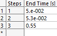
Figure 3. End time of three steps.

Gravity is defined as a time-dependent acceleration accordingly, as shown in Figure 4. Essentially, gravity is not activated from 0s to 0.05s. From 0.05s to 0.053s, gravity is ramped from 0 to g. After 0.053s, gravity is maintained as g.

Figure 4. Scheduling gravity activation by step.

As a result, the impact and rebound are simulated successfully. The impact velocity in the simulation is slightly higher than 2.6943m/s as the gravity is ramped from 0 to g in 0.003s and maintained as g in 0.0047s before the impact, but the influence is negligible. The results can be refined by further reducing the time window for gravity activation.