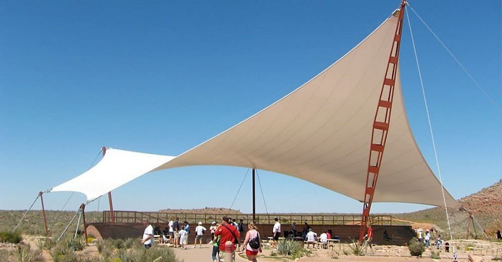
Fig.1. A typical cable-membrane structure
The following assumptions are made in this example:
- Cables are discretized using LINK10 elements. The membrane is discretized using triangular SHELL41 elements with ‘cloth’ feature turned on.
- No slip between cables and membrane.
- The material complies with Hooke’s Law.
- The material is orthotropic and elastic. The two principal axes of the material remain orthogonal before and after deformation.
The desired shape in this example:
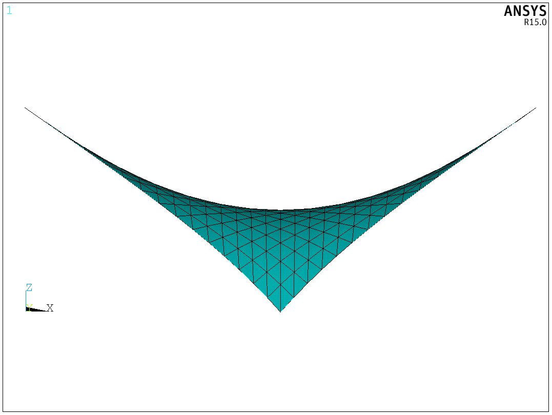
Fig.2. Front view
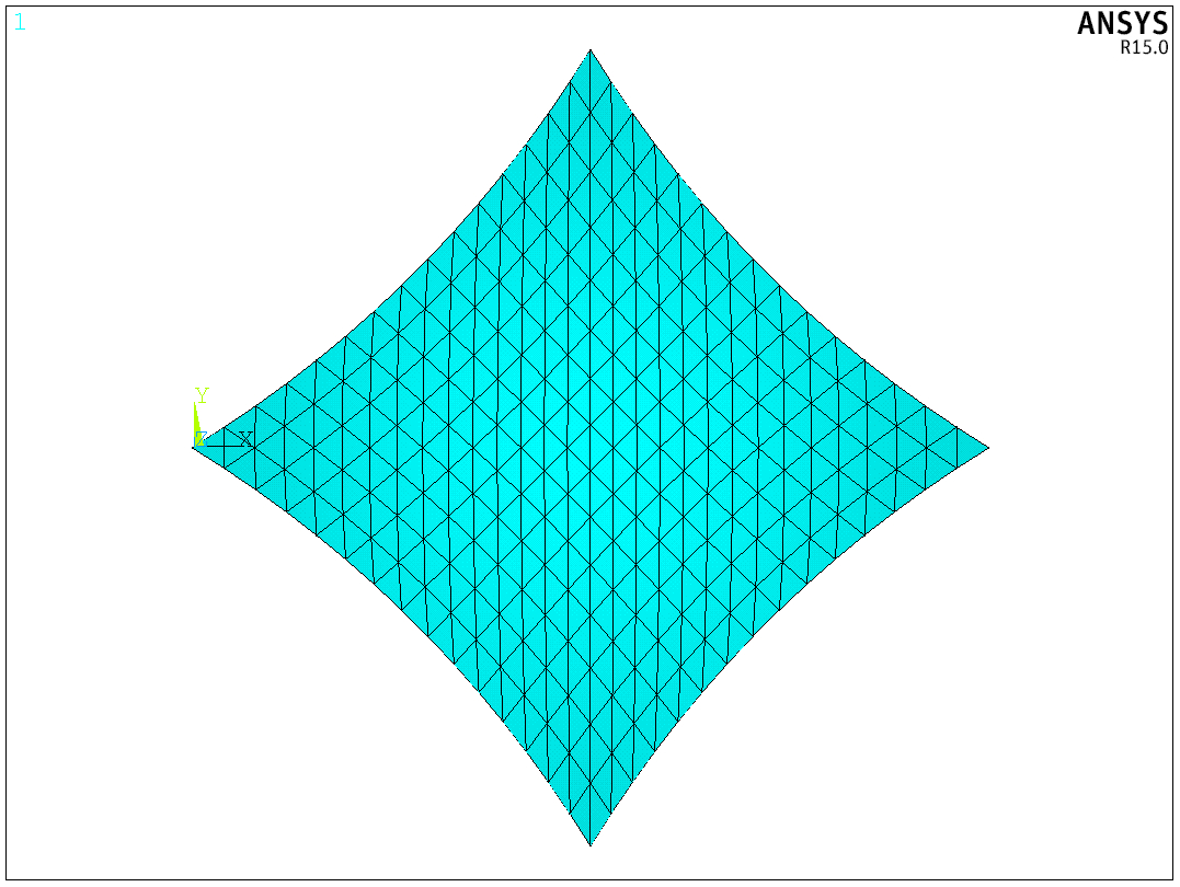
Fig.3. Vertical view
Shape-finding is essentially a static equilibrium problem. In this example, the process of shape-finding is as follows:
- Create the geometry of the planar projection of the cable-membrane structure.
- Assume dummy elastic modulus values for the membrane and cable. In this example, the dummy values are 1/1000 of the true values.
- Define element type, real constants, and prestress. The prestress in cables are achieved through initial strain (defined in real constants). The prestress in the membrane is achieved through cooling method. Thus the thermal expansion coefficient of membrane material should be defined.
- Mesh the model.
- Define boundary conditions. Set the lifting displacement of each support.
- Perform shape-finding. Update nodal coordinates. Change the lifting displacement to zero.
- Define the true elastic modulus. Reset the parameters of prestress based on the true values of elastic modulus.
- Perform the first iteration. Repeat steps 5 to 7 for multiple times, until converged results are reached. The final shape is found.
The APDL for shape-finding and static analysis:
FINISH
/CLEAR
!units: N, m, Pa

/PREP7
ET,1,SHELL41
MP,EX,1,2.55E5		!dummy elastic modulus
MP,PRXY,1,0
MP,ALPX,1,10		!applying prestress to the membrane using cooling method
KEYOPT,1,1,2		!'cloth' option
TREF,0
ET,2,LINK10
MP,EX,2,1.5E8		!dummy elastic modulus
MP,PRXY,2,0.3
R,1,0.001			!thickness of the membrane
R,2,0.0002,0.99999		!cross-sectional area and initial strain (must be <1.0) of the cable

K,1
K,2,10
K,3,5,5
K,4,5,-5
A,1,3,2,4

LSEL,ALL
LATT,2,2,2
ASEL,ALL
AATT,1,1,1
LESIZE,ALL,,,15
MSHAPE,1,2D
MSHKEY,1
ASEL,ALL
AMESH,ALL
LSEL,ALL
LMESH,ALL

DK,1,ALL
DK,2,ALL
DK,3,ALL
DK,4,ALL
DK,1,UZ,4
DK,2,UZ,4
ASEL,ALL
BFA,ALL,TEMP,-0.7843

/SOLU
ANTYPE,0
NLGEOM,ON		!SSTIF will be turned on if NLGEOM,ON
NSUBST,10
CNVTOL,F,,0.01
LNSRCH,ON
ALLSEL
SOLVE

/POST1
PLNSOL,S,EQV
UPCOORD,1,0		!modifies the coordinates of the active set of nodes, based on the current displacements. If FACTOR = 1.0, the full displacement value will be added to each node
ESEL,S,TYPE,,1
*GET,MINNUM,ELEM,0,NUM,MIN
*GET,MAXNUM,ELEM,0,NUM,MAX
J=0
*DO,I,MINNUM,MAXNUM
*GET,T,ELEM,I,AREA	!get the area of area element
J=T+J
*ENDDO			!J is the area of the membrane

/PLOPTS,INFO,2
/PLOPTS,LEG1,0
/PLOPTS,LEG2,0
/PLOPTS,TITLE,0
/PLOPTS,MINM,0
/PLOPTS,FILE,0
PRRSOL			!prints the constrained node reaction solution
/PREP7
MP,EX,1,2.55E8		!real elastic modulus
MP,ALPX,1,0.01
MP,EX,2,1.5E11		!real elastic modulus
R,2,0.0002,0.001		!real prestrain in the cable. Strain=F/EA
/SOLU
DK,1,ALL
DK,2,ALL
DK,3,ALL
DK,4,ALL
ALLSEL
SOLVE

UPCOORD,1,0
/POST1
ESEL,S,TYPE,,1
*GET,MINNUM,ELEM,0,NUM,MIN
*GET,MAXNUM,ELEM,0,NUM,MAX
J=0
*DO,I,MINNUM,MAXNUM
*GET,T,ELEM,I,AREA	!get the area of area element
J=T+J
*ENDDO			!J is the area of the membrane
/PLOPTS,INFO,2
/PLOPTS,LEG1,0
/PLOPTS,LEG2,0
/PLOPTS,TITLE,0
/PLOPTS,MINM,0
/PLOPTS,FILE,0
PRRSOL

*DO,I,1,3
ALLSEL
/SOLU
SOLVE
UPCOORD,1,0
*ENDDO

/POST1
ESEL,S,TYPE,,1
*GET,MINNUM,ELEM,0,NUM,MIN
*GET,MAXNUM,ELEM,0,NUM,MAX
J=0
*DO,I,MINNUM,MAXNUM
*GET,T,ELEM,I,AREA	!get the area of area element
J=T+J
*ENDDO
PRRSOL

!define loads and solve
/SOLU
ALLSEL
NSEL,ALL
F,ALL,FZ,108
NSUBST,15
CNVTOL,F,,0.025
LNSRCH,ON
OUTRES,ALL,ALL
MP,DENS,1,1050
MP,DENS,2,7850
ACEL,,,9.8
ALLSEL
SOLVE

/POST1
PLNSOL,S,EQV
PRRSOL

/SOLU
NSEL,ALL
F,ALL,FZ,0		!overwrite the previously defined load
LSWRITE,1
NSEL,ALL
F,ALL,FZ,24
LSWRITE,2
NSEL,ALL
F,ALL,FZ,48
LSWRITE,3
NSEL,ALL
F,ALL,FZ,72
LSWRITE,4
NSEL,ALL
F,ALL,FZ,108
LSWRITE,5
NSEL,ALL
F,ALL,FZ,180
LSWRITE,6
OUTPR,ALL,LAST
OUTRES,ALL,LAST
RESCONTROL,,NONE,NONE
LSSOLVE,1,5

/POST1
PLNSOL,U,Z
PLESOL,S,1
PLESOL,S,2
AVPRIN,0, ,
ETABLE,ZL,LS,1
PLETAB,ZL,AVG
PLLS,ZL,ZL,1,0  		!draw the axial force diagram of cables

/POST26
NSOL,2,141,U,Z,UZ2
NSOL,3,160,U,Z,UZ3
NSOL,4,166,U,Z,UZ4
NSOL,5,256,U,Z,UZ5
PLVAR,2,3,4,5
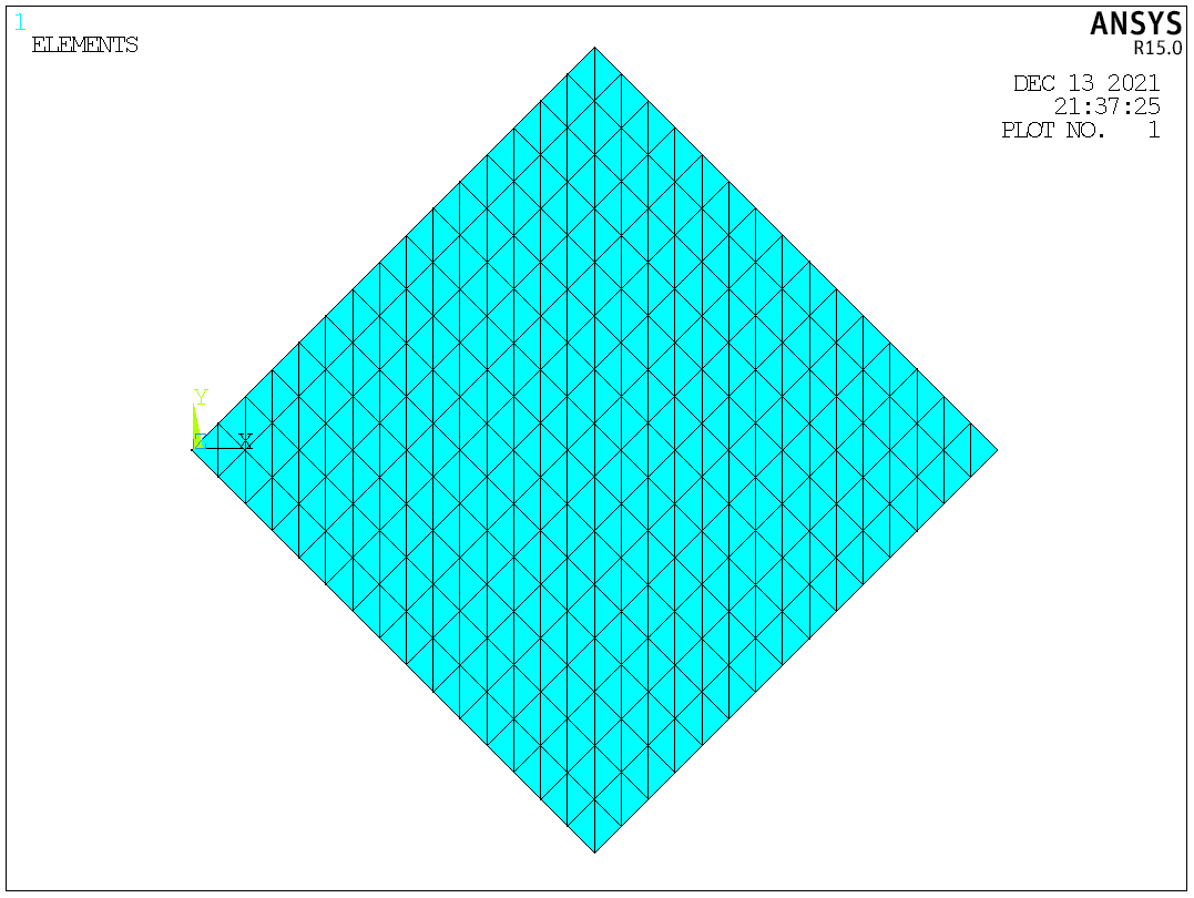
Fig.4. The planar projection of the cable-membrane structure
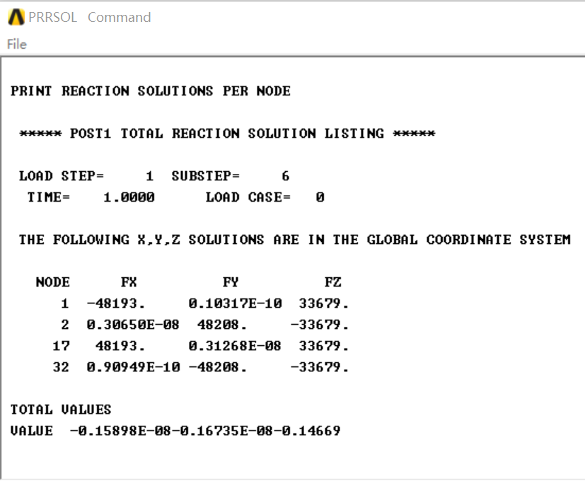
Fig.5. The reaction solution after iterations

Fig.6. Von Mises stress solution after iterations. The stress distribution is relatively uniform.
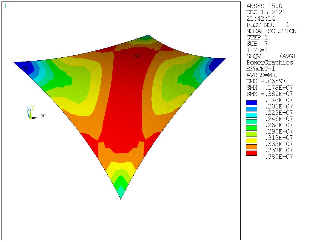
Fig.7. Von Mises stress solution after loading
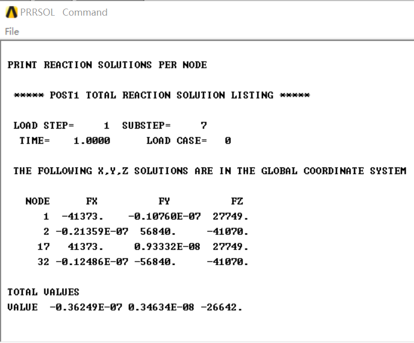
Fig.8. The reaction solution after loading

Fig.9. The axial force diagram of cables
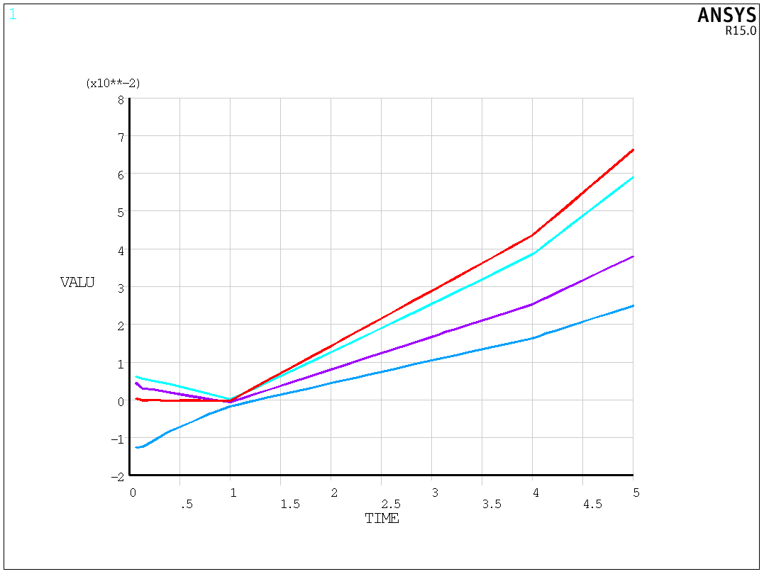
Fig.10. The curves of displacement vs. load
Modal analysis is based on the shape obtained after shape-finding. However, a static analysis is carried out first with large deflection turned off and stress stiffening turned on. After the shape-finding, the APDL for modal analysis is as follows:
/SOLU
ANTYPE,0
NLGEOM,OFF
SSTIF,ON
LUMPM,ON
MP,DENS,1,1050
MP,DENS,2,7850
ACEL,,,9.8
ALLSEL
SOLVE
FINISH

/SOLU
ANTYPE,MODAL
NSEL,ALL
DDELE,ALL,ALL
DK,1,ALL
DK,2,ALL
DK,3,ALL
DK,4,ALL
ALLSEL
MODOPT,LANB,12
MXPAND,12
LUMPM,ON
PSTRES,ON
SOLVE

/POST1
SET,LIST
SET,1,1
PLNSOL,U,Z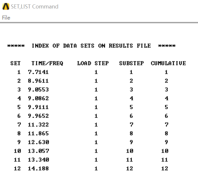
Fig.11. The first twelve natural frequencies

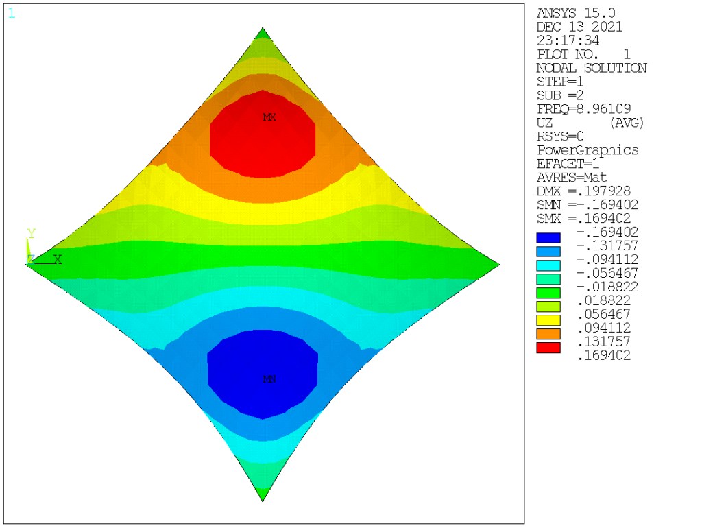

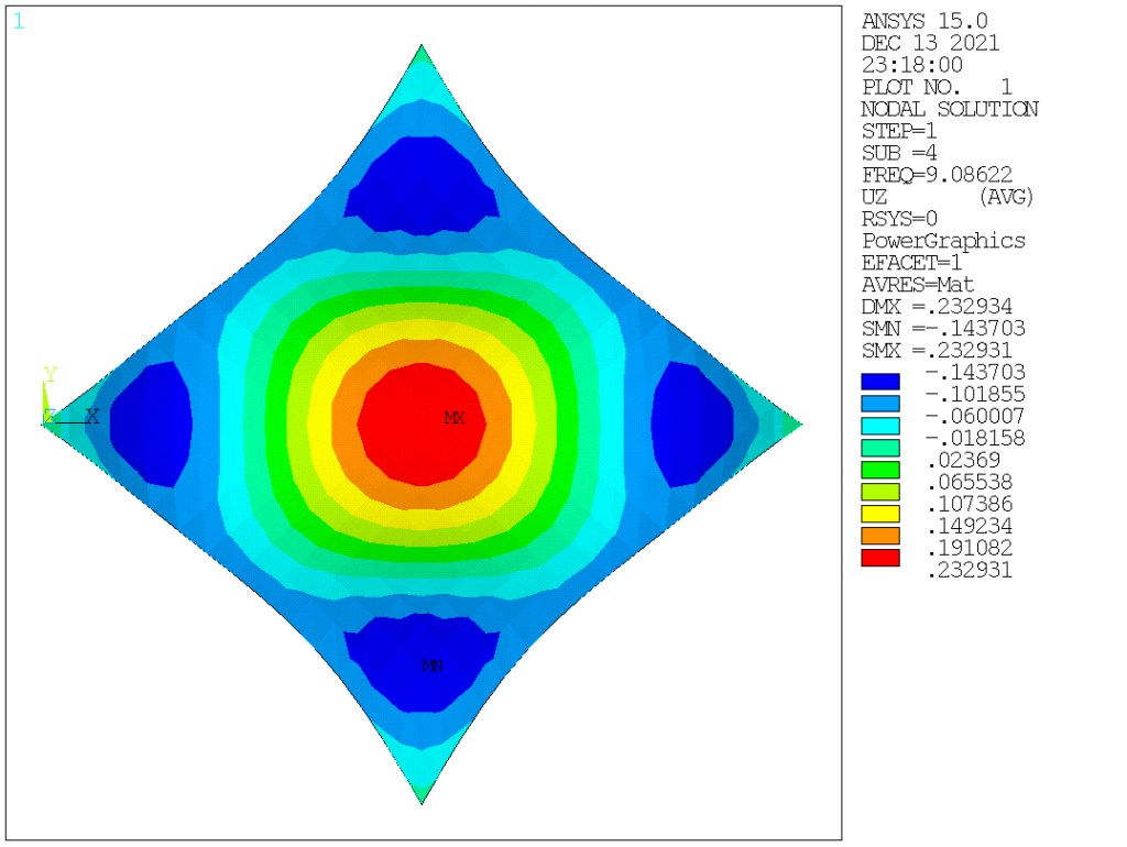
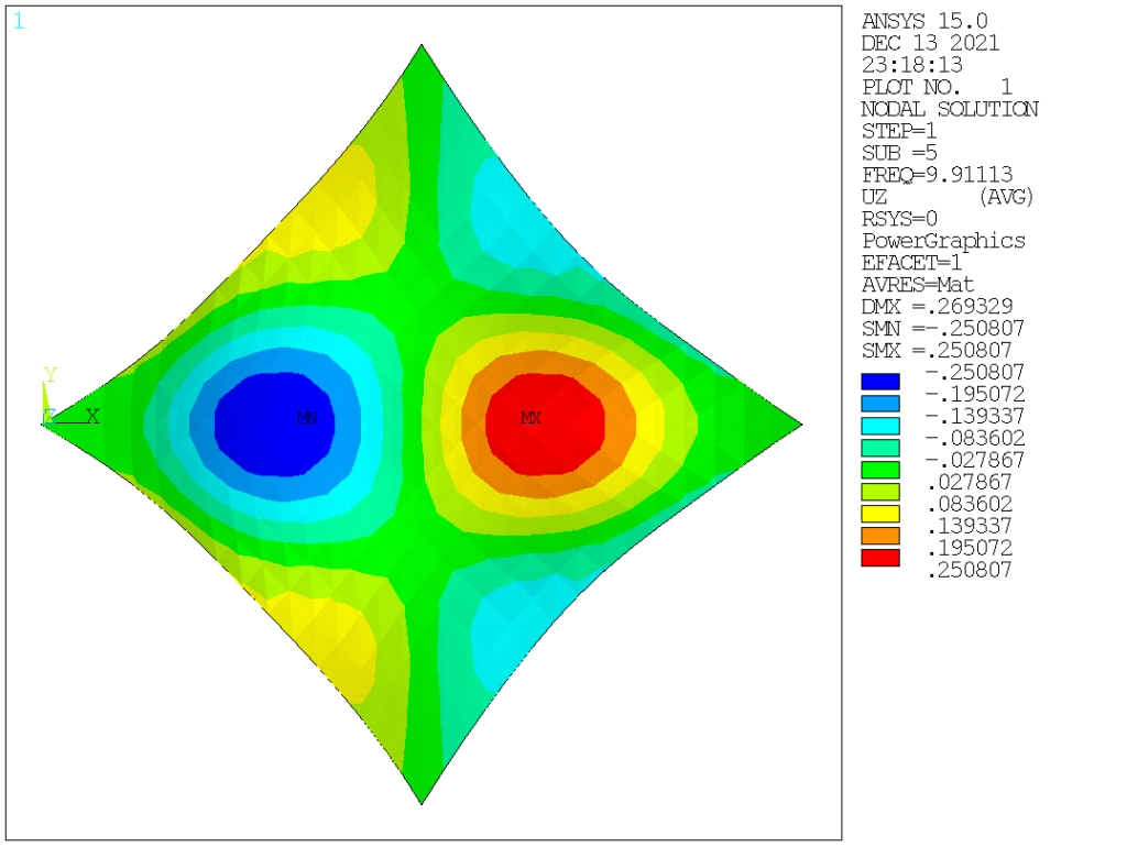
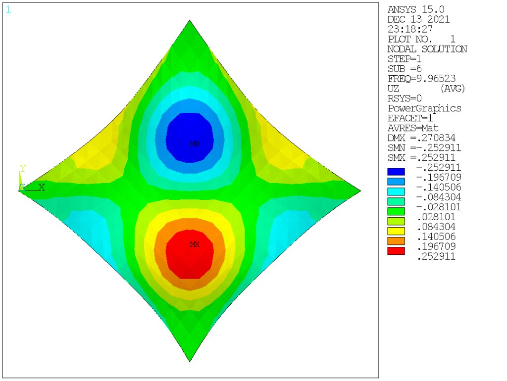
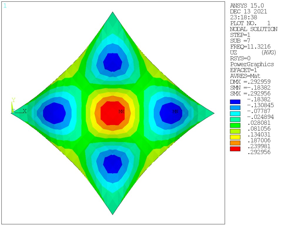

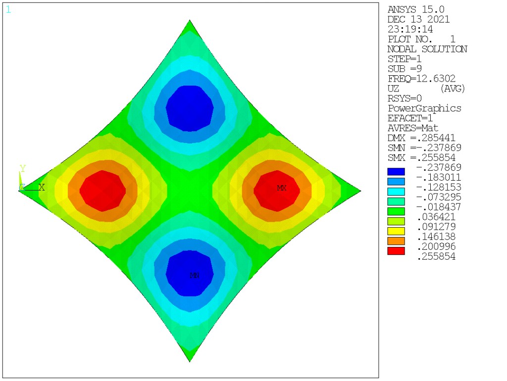

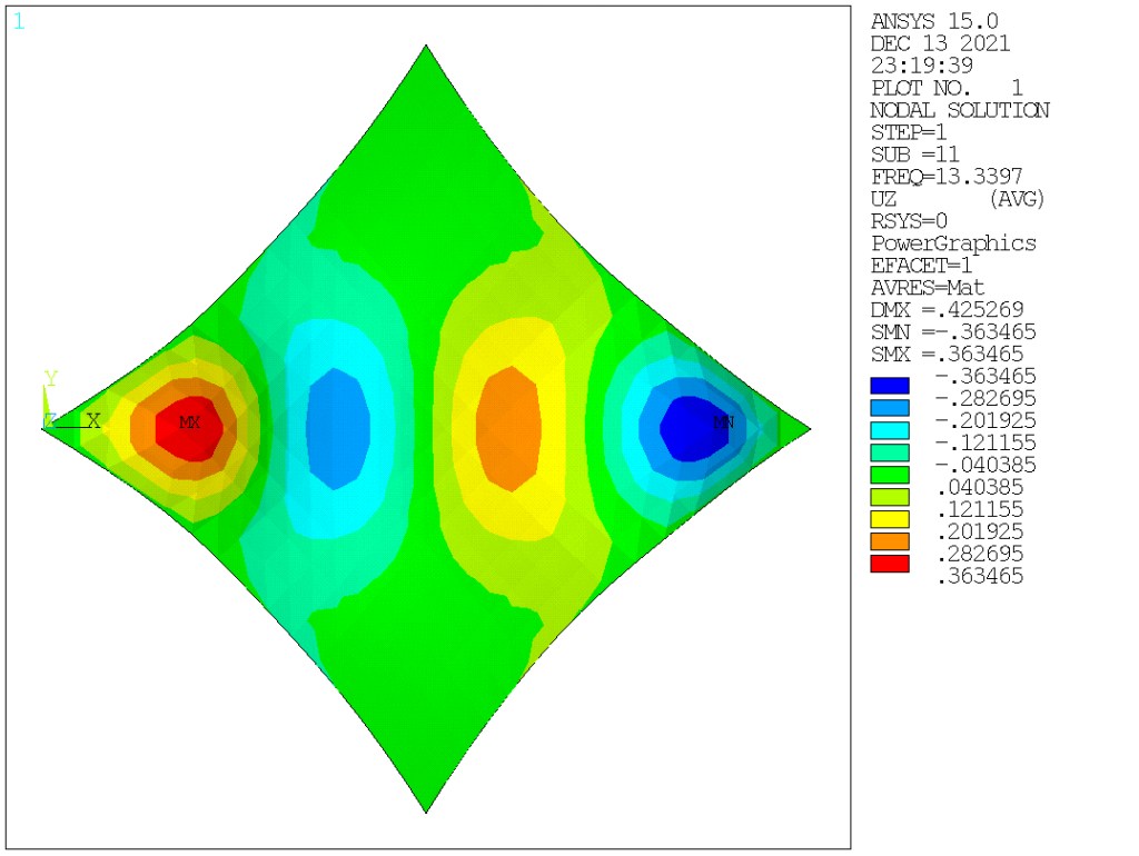

Fig.12. The first twelve mode shapes
