Any loading can be understood as transient, but it can also be understood as a spectrum of waves. Treating dynamic problem inputs and outputs as a combination of waves (or wave spectrum) simplifies the problem by removing the concept of time. However, the solution is approximate and with certain limitations.

You can use a response spectrum analysis rather than a time history analysis to estimate the response of structures to random or time-dependent loading environments such as earthquakes, wind loads, ocean wave loads, jet engine thrust or rocket motor vibrations.

Just like transient shock analysis and harmonic response analysis, a free vibration analysis is needed beforehand to calculate natural frequencies. Also it is important to ensure the mesh is sufficient to describe the highest mode shape, and the 80% mass participation criteria should be satisfied in most cases (see this post).

What do we mean by Response Spectrum?

In a typical case where the response spectrum is specified for base acceleration, the acceleration response spectrum graph is shown here.

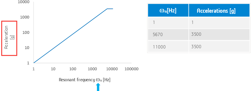
We can see the spectrum is specified in the frequency domain, not time domain. Contrary to the harmonic analysis where the frequency means the operating frequency of some loading force, here the horizontal axis is the natural frequency ωn of a series of single-degree-of-freedom (SDOF) systems.

How to generate the acceleration response spectrum?

The response spectrum is fundamentally derived from a series of SDOF systems. A response spectrum shows the maximum response of many different SDOF systems subjected to the same ground motion. As an example, a SDOF oscillator is subjected to a base excitation a as a function of time.

The base excitation, however, is not an easy load. In fact, very complex loading environments such as earthquakes are typical. Attempting to solve such complex histories in time using transient dynamic simulation would be extremely difficult and in many cases impractical. Response spectrum method makes solution of such a complex environment much easier.

Taking advantage of the fact that the oscillator is as simple as it can get, we can obtain its response acceleration, a, of mass for the load of any complexity. Of course, because loads as complex as those shown here are only available in the form of discrete measured data, solutions are also obtained using numerical methods.

The last important point before moving on to the response spectrum is to identify a quantify characterizing the system, i.e. SDOF oscillator. Knowing its stiffness k and mass m, one would naturally select its natural frequency ωn, calculated from these two values. We are now ready to generate the acceleration response spectrum.

As shown in the following graph, we will plot the natural frequency of the oscillator ωn. We will start with a randomly selected natural frequency ωn1 simulating an oscillator of certain stiffness k and mass m. We will then employ numerical methods and obtain solution to the complex base motion. Instead of retaining all the complex solution, however, we will only retain the response amplitude A1. In other words, we will note the largest acceleration response of the oscillator in this graph. This will give us the first point in the response spectrum.

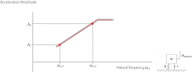
Then we choose a different natural frequency of the oscillator, solve the complex problem, and again note the acceleration amplitude of the oscillator response in the graph. We will repeat the process for many randomly selected natural frequencies of the oscillator response, until we have enough data point to plot a graph.

The vertical axis therefore contains amplitude of the acceleration response of the oscillator, horizontal axis covers a range of oscillators, or more specifically, their natural frequencies.

We now constructed the acceleration response spectrum. The good news is that the tools to create such response spectrum are readily available.

Also notice that any information about when this acceleration amplitude occurs is lost. Response spectrum only shows the extreme acceleration response of the oscillator, but we do not know when it occurred. From the engineering perspective, amplitudes of the response are important because these extreme values are important for our designs.

To summarize, response spectrum contains information about the load, because this is how it is designed. In fact, it contains more than that. It contains the solution, or the response of the oscillator to the dynamic loading. Because response spectrum contains amplitude of the oscillator response to the dynamic loading, all time information and phase angles are lost. Besides, all results such as displacements, velocities, accelerations, stress, etc. must be understood as amplitudes, or the largest response that occur on the model.

Response Spectrum study properties in SolidWorks Simulation

Response spectrum study properties are different form the properties of the harmonic and transient study types. Because response spectrum lacks the time information for when the amplitudes of the response occur, summations of the modal solutions to get the overall response of the model cannot be done accurately. Instead, several mode combination methods for summing modal solutions have been devised.

Square Root Sum of Squares (SRSS) estimates the peak response by the square root of the sum of the maximum modal responses squared.

Absolute Sum assumes that maximum response of the modes occur at the same time. It is the most conservative among the modal combination methods.

Complete Quadratic Combination (CQC) is based on random vibration theories. It is recommended for simulations involving seismic loads.

Naval Research Laboratory (NRL) method takes the absolute value of the response for the mode that exhibits the largest response and adds it to the SRSS response of the remaining modes.

Selection of the method is driven by the standard you need to follow or by given requirements.   

Curve interpolation option controls how to interpolate the data in the response spectrum curve.