Random vibration analysis is useful in solving complex vibration problems. Examples of non-deterministic loads include:

• Loads generated on the wheel of a car travelling on a rough road
• Base accelerations generated by earthquakes
• The pressure generated by air turbulence
• Pressure from sea waves or strong wind

Random vibration analysis provides probabilistic information about output such as displacements, velocities, accelerations, and stress. Random vibration study assumes Gaussian distribution of the input signal such as measured acceleration. Input in random vibration study is in the form of so-called power spectrum density function, typically for acceleration. While units and values of this function may appear rather abstract, it provides a powerful, yet easy way to understand the severity of the vibratory environments. That is the reason why this input is preferred as opposed to the transient input, which can be exceedingly complex. Similar to other spectral methods, time information about when the amplitudes occur is lost.

In this post, we are going to talk about a few concepts in random vibration analysis. We are not delving into the mathematical level, but understanding these concepts is crucial to implementing the analysis and interpreting results correctly.

Complex transient loading

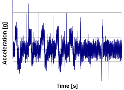
All vibratory environment characteristics start with some more or less complex transient signal obtained from real measurements. This example can be a measured acceleration caused by an earthquake, or vibration inside an automobile or airplane.

Random vibration loading

Similar to response spectrum analysis, random vibration analysis decomposes the complex transient loading into the spectrum of waves. It therefore solves the problem in the frequency domain, rather than the time domain. However, the input is in the form of so-called power spectral density curve or PSD. As a typical example, when the PSD curve is specified for base acceleration as shown in the following graph, we can call it PSD of acceleration.

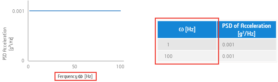
Notice that the unit of PSD of acceleration is g²/Hz. Contrary to the response spectrum analysis, and similar to harmonic response analysis, random vibration PSD spectrum is specified in terms of the exciting frequency of the load, and not the natural frequency of the structure.

Gaussian distribution

While various distribution models exist, random vibration simulation assumes the most common Gaussian, or Normal distribution.

Now the first question is what is meant by the distribution of this signal?

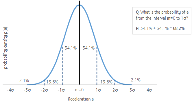
In this distribution, the probability density ρ is for any variable, and the acceleration a is the famous bell curve. The curve is centered around the mean value m. In engineering simulations, we always assume that m is equal to 0.

Another important statistical constant is statistical deviation σ, indicating how dispersed the measured accelerating signal values are from its mean m. In the graph, we can show statistical deviation σ, here denoted as 1σ, and its multiples 2σ, 3σ, 4σ and so forth on both sides of the mean, until whatever multiple value required by a technical standard we need to satisfy. For engineering use, we need to understand the probability of acceleration a assuming a value within a certain interval.

A typical question is: What is the probability of acceleration a assuming a value from 0 to 1σ?

To calculate probability, we need to integrate this bell curve, or in other words, we need to calculate the area under the bell curve for this specific interval. Theoretically, the answer to our question is 34.1%. However, because we consider random vibration along the positive or negative direction equal, we will calculate the area all the way from the negative 1σ to positive 1σ, i.e. 68.2%. In other words, variable x will assume values from the negative 1σ to positive 1σ for 68.2% of time. The probabilities for the remaining intervals are of course incrementally smaller and are shown in the above graph.

Root mean square (RMS)

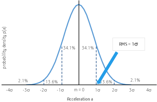
The second important value we use in engineering calculation is Root Mean Square, or RMS. With the mean value m equal to zero, RMS is equal to 1σ statistical deviation. A different way to explain the RMS value is to think of it as the averaged value of the amplitude of the acceleration signal. The important fact is that the probability of the acceleration reaching amplitudes between zero and the RMS value is 68.2%.

Power spectral density

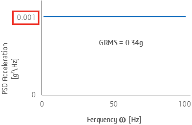
Now let’s look at some important characteristics of power spectral density function. As shown in the following example, the value of the PSD curve here is 0.001g²/Hz. In rather simplified and non-exact terms, we can look at this value as some kind of power of the vibratory environment at a given frequency. 0.001g²/Hz is a rather mild environment. Values close to 1g²/Hz are severe environments that are deadly to humans. As a consequence, the height of the PSD curve indicates the power of the vibration at a given frequency. One can therefore look at PSD and read similar information from it as one would get from FFT. If the value is high, the power of those particular waves in the signal is strong, and vice versa.

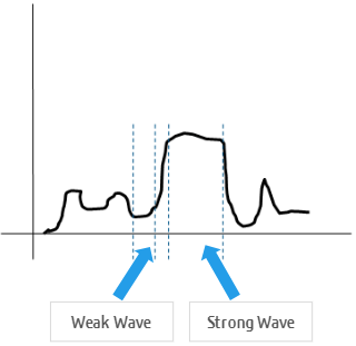
We can take the following PSD curve as an example. The values of the PSD curve are small in the first band, therefore the waves in the first band are weaker and contribute less to the overall measured acceleration signal. Contrary to that, waves in the second band are strongly present in the measured signal.

Now let’s come back to the previous PSD curve showing 0.001g²/Hz. The most important characteristic of PSD is that when we integrate the PSD curve across the frequency range, we will get the RMS value of the signal. Because acceleration is commonly referred to in the unit of g, this RMS value is denoted as GRMS. In the example, integrating the PSD curve will result in GRMS of 0.34g. Now we can conclude that some average acceleration in the environment specified by this PSD curve is 0.34g, which is rather small. And because RMS is equal to 1σ, any object exposed to this environment will feel 0.34g or smaller acceleration levels for 68.2% of time.

Power Spectral Density vs. Transient Signal

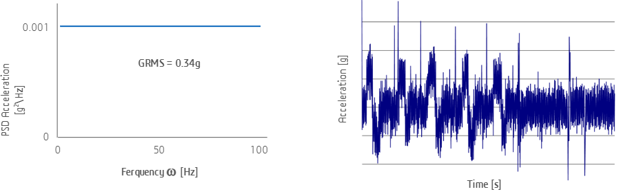
From the above analysis, we can conclude that the level of the PSD curve (i.e. 0.001g²/Hz) and the GRMS value of the acceleration (i.e. 0.34g) are rather small. This vibratory environment is therefore not severe. However, it would be difficult to judge how severe the environment is if simply by looking at the transient signal. We can read some peak accelerations, but the wave content is entirely hidden to a naked eye. This highlights the advantage of solving dynamic problems in frequency domain because transient histories are not convenient for easy judgement of how severe the vibratory environments are.

Furthermore, there can be multiple similar transient signals with the same PSD function. PSD function therefore provides extremely powerful and clean insight into the severity of the vibratory environment. For experimental purposes, knowing PSD curve, it is always possible to synthesize a transient history, which is then fed directly to a shaker table to produce real vibrations in time.

How to post-process random vibration analysis?

Post-processing of random vibration study involves reviewing two types of output:

• RMS output, which provides information about amplitudes at 1σ statistical deviation levels. Amplitudes at higher level such as 2σ, 3σ, or higher, are easily obtained by multiplying the RMS values (1σ level values) by 2, 3, etc. Each higher level comes at a higher probability, but with increased cost. At higher σ levels, the increase in probability and safety of the design is rather small, but the corresponding increase in cost is exponential.
• PSD output, which provides information about the wave content of the output. In other words, PSD curve provides insight into at what frequencies the output location would predominantly oscillate, and what is the overall strength of the output vibration.