A wind turbine blade is a long, hollow structural component made of composite material. Due to its slender nature, it is important to conduct a buckling design test to prevent such failure in service. This post illustrates how to use Ansys ACP to set up composite materials and apply them to wind turbine blade buckling analysis. Specifically, we will introduce several important concepts in Ansys ACP and the general workflow of composite simulation using ACP and Mechanical.

As shown in Figure 1, the blade is modeled using two solid parts (i.e. stiffeners) and one shell part (i.e. blade body), however, the composite material is only applied to the shell part. Therefore, solid parts should be suppressed before creating a composite blade using ACP.

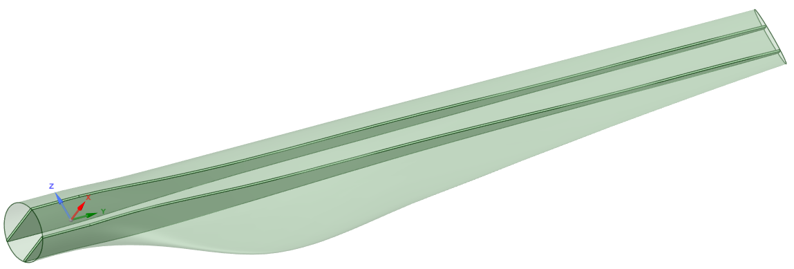
Figure 1. Blade geometry

Figure 2 shows the workflow of this simulation. The shell part and solid parts are meshed separately and assembled later in the static analysis. Before entering the ACP environment for composite creation, the shell part has been meshed (see Figure 3).

Figure 2. Data transfer in Workbench

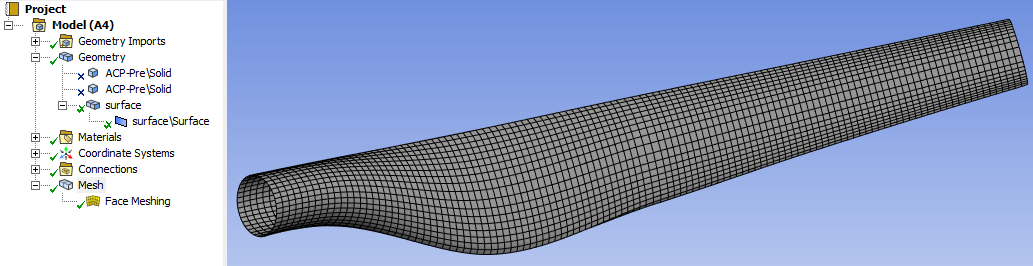
Figure 3. Shell mesh.

Once entering ACP, the first step is to define the material data. Materials are carried over from the Engineering Data. Fabrics and Stackups can be easily customized (see Figure 4).

Fabrics in ACP

Fabrics represent the raw material (e.g., woven or unidirectional carbon fiber/epoxy) and define the mechanical properties and thickness of one material layer. They are the fundamental building block of a laminate. They are used to define individual plies or as components within a stackup. 

Stackups in ACP

Stackups are predefined arrangements of multiple fabrics with specific orientations and stacking sequences (e.g. [0/45/90]𝑠). They simplify the layup process, making it easier to apply complex, repeated laminate sequences. They are used when a specific sequence of layers is consistently used throughout the design, or to define sandwich structures by combining core materials. 

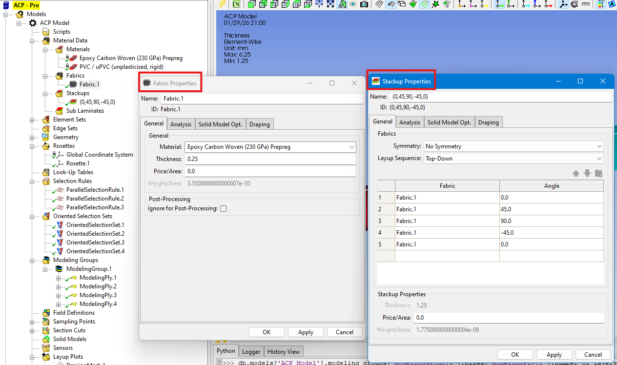
Figure 4. Define fabric properties and stackup properties.

Define Rosettes

Rosette is another important concept in ACP. Essentially, it refers to a local coordinate system used to define the 0-degree reference direction for composite ply orientations and layups. To define a typical parallel rosette, an origin and two directions are needed (see Figure 5). A schematic explanation of the two directions is given in Figure 6 where the red axis (i.e. x axis, direction 1) aligns with the 0-degree direction and the blue axis (i.e. z axis, direction 2) aligns with the 90-degree direction.

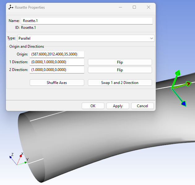
Figure 5. Defining a rosette.

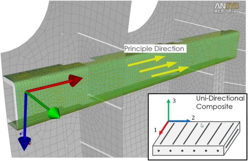
Figure 6. Rosette directions (source).

Define Selection Rules

Selection Rules in ACP are used to define localized ply shapes, reinforcements, or cut-outs by selecting elements based on geometric criteria rather than direct mesh selection. They allow for local reinforcement patches, staggering, and handling cut-outs (e.g. windows) without requiring complex, pre-split CAD geometry. They are fully parametric, meaning they update automatically with changes in geometry. They are applied to Oriented Selection Sets or Modeling Plies (which are introduced below) to precisely define where materials are applied.

In this example, the thickness varies along the blade because different numbers of stackups are applied up to various lengths (see Figure 7 and Figure 8).

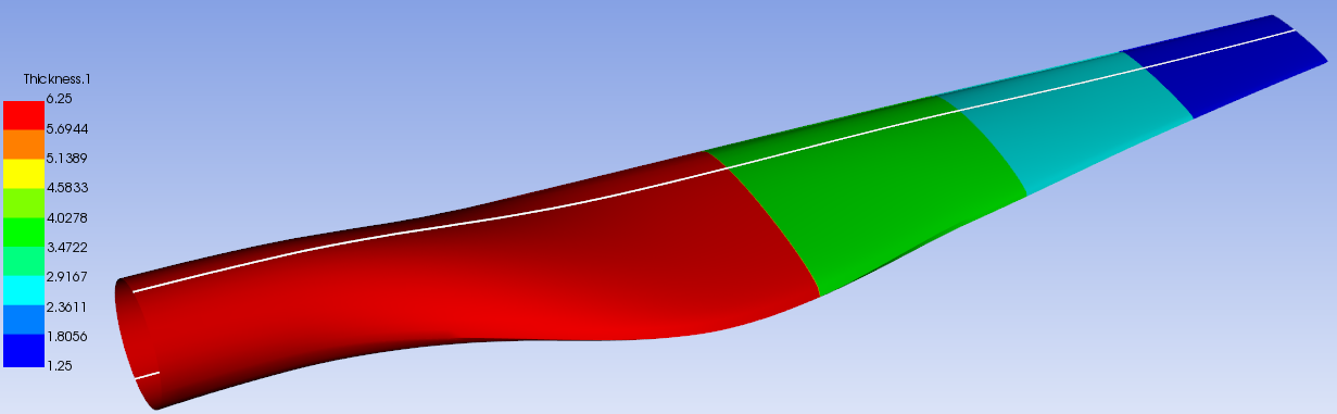
Figure 7. Thickness plot.

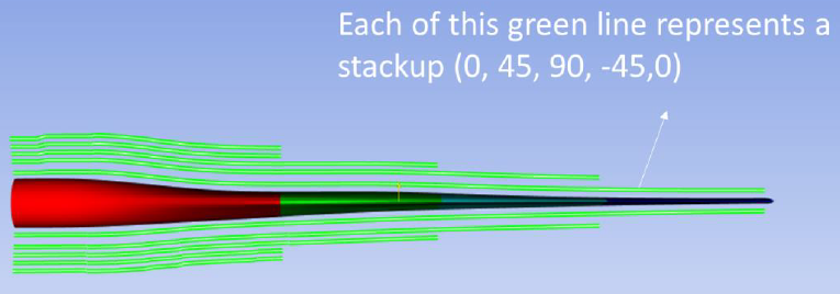
Figure 8. Stackup variations along the blade.

To control the various regions for different numbers of stackups, three parallel selection rules are defined (see Figure 9).

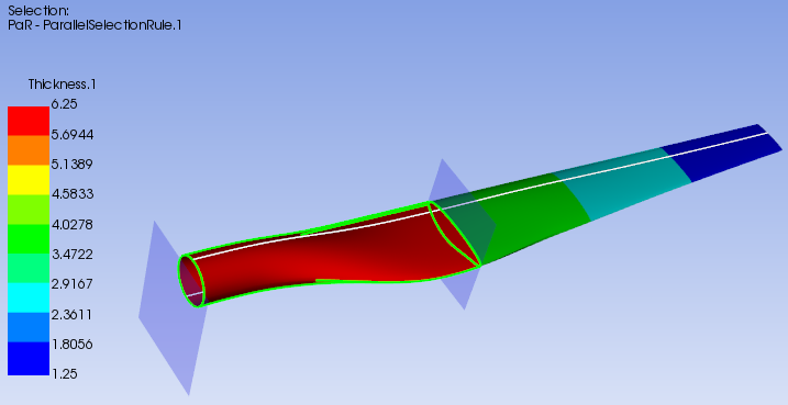
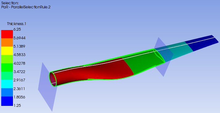
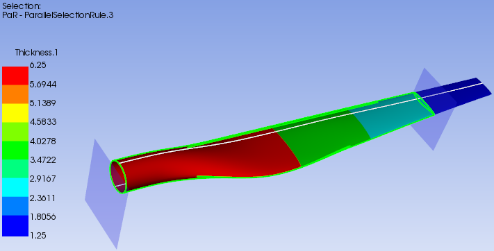
Figure 9. Parallel selection rules.

Figure 10 shows a typical definition of a parallel selection rule. The region for selection is defined with respect to the picked origin, local axis direction, and lower/upper limits. Next, selection rules are applied to Oriented Selection Sets and Modeling Plies.

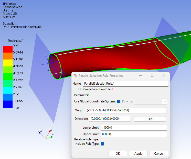
Figure 10. Parallel selection rule definition.

Define Oriented Selection Sets

Oriented Selection Sets (OSS) define the foundational orientation, stacking direction, and spatial location for composite plies on a mesh. As shown in Figure 11, an OSS combines a specific element set (the mesh area), a rosette (to define the 0-degree reference direction), and a thickness direction (defining which way the layup grows, i.e. top or bottom). It bridges the gap between geometric surfaces and finite element nodes. Plies are applied to OSS, not directly to raw mesh elements. It defines the stacking direction, which can be flipped to ensure the layup grows in the correct direction (e.g. into the mold).

OSS are essential for organizing complex models with different ply regions. They are created after defining elements and rosettes, often using named selections from Mechanical to define the target area. 

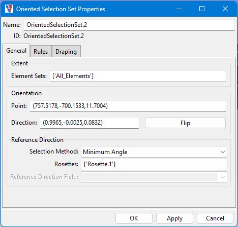
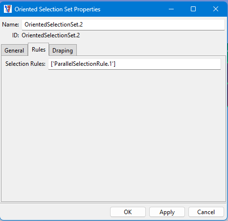
Figure 11. Set OSS properties.

Define Modeling Groups

Modeling Groups are used to create, organize, and stack modeling plies (see Figure 12), which define the material, thickness, and orientation of composite layers. Modeling groups use Oriented Selection Sets to map the material definitions onto the actual FE model, ensuring proper fiber orientation and direction. They enable the visualization of fiber orientation, thickness, and the overall stacking sequence of the composite structure (e.g. Figure 8). 

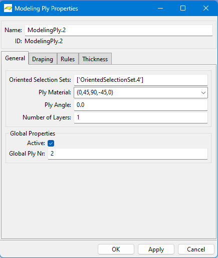
Figure 12. Set modeling ply properties.

After meshing the shell part and solid parts separately, the model data is transferred to the static analysis, where bonded contacts are detected and applied automatically, and the mesh is inherited from ACP(Pre) and Mechanical Model (see Figure 13).

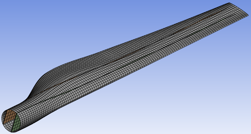
Figure 13. The final mesh.