The Eigenvalue Buckling analysis in Workbench takes the results of a Static Structural analysis and calculates the load multiplier that would cause a structural buckling. If in the Static Structural analysis, loads and gravity are applied together to take into account the self-weight of the structure, then the buckling multiplier would also ‘multiply’ the gravity, which is a non-physical situation.

There are two workflows to handle this situation.

Workflow #1: Buckling solution iteration

Consider the example of a column with a self-weight W₀ and an externally applied load A as shown in Figure 1. Instead of applying unit load A=1.0, users may iterate on the buckling solution, adjusting A until the load multiplier becomes 1.0 or nearly 1.0. From Figure 1, A is gradually increased from 1 to 111 until λ equals 0.99, so that the final load leading to buckling is F=0.99*111+0.99* W₀

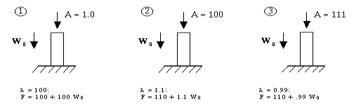
Figure 1. Adjust load A until λ approaches 1.0

In Ansys Workbench, the workflow will look similar to a common Eigenvalue Buckling analysis (see Figure 2). The only difference is that gravity is now considered in the Static Structural analysis, and the applied load is not a unit load. In fact, the applied load should be adjusted so that the load multiplier is close to 1.0.

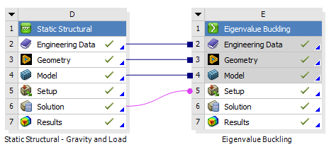
Figure 2. Workflow #1

Workflow #2: Buckling analysis on the deformed geometry

In the second workflow, Static Structural analysis #1 is performed with gravity applied only. Then Static Structural analysis #2 is performed on the deformed geometry, with the unit load applied. Finally, the results are transmitted to the Eigenvalue Buckling analysis to calculate the load multiplier. This process is shown in Figure 3.

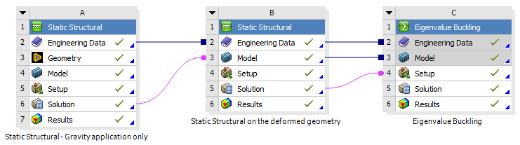
Figure 3. Workflow #2

Example

In this example, we have a 2-meter-long steel cantilever box beam subject to self-weight and a force on the free end, as shown in Figure 4.

When taking workflow #1, the applied force is changed from 1N to 57718N, so that the load multiplier decreases from 254.62 to 0.9962. The final load leading to buckling is F=0.9962*57718+0.9962* self-weight. The buckling mode is shown in Figure 5.

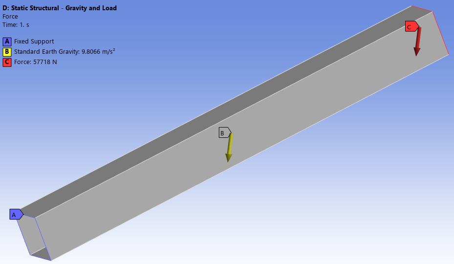
Figure 4. Load and BCs (workflow #1)

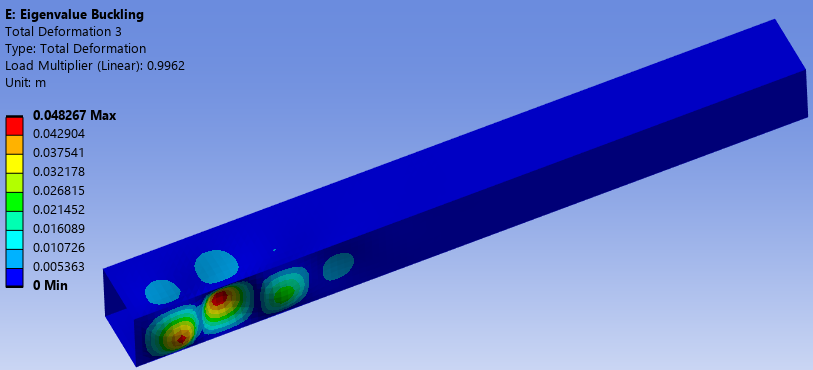
Figure 5. Buckling mode (workflow #1)

When taking workflow #2, the gravity is applied in the first Static Structural analysis (see Figure 6), then a unit load is applied in the second Static Structural analysis (see Figure 7). The load multiplier is calculated to be 57718, which means the final load leading to buckling is F=57718*1+self-weight. The buckling mode is shown in Figure 8, which is practically identical to Figure 5.

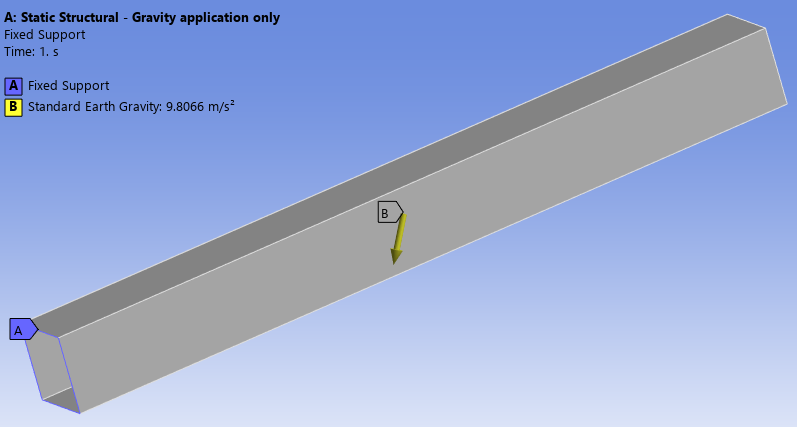
Figure 6. Load and BCs (gravity applied only)

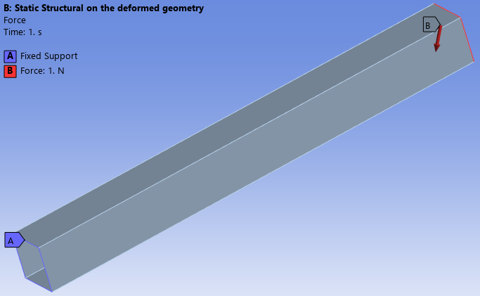
Figure 7. Load and BCs (apply a unit load on the deformed shape)

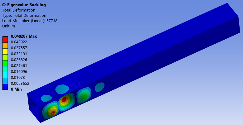
Figure 8. Buckling mode (workflow #2)

Overall, the above example indicates that both workflows deliver the same results, and users can apply their own judgment regarding which workflow is more compatible with their practice.