Laser welding is a highly localized heat input process in which a moving heat source induces steep thermal gradients. These gradients lead to thermal expansion and contraction generating residual stresses. They may also cause material softening or phase changes in the heat-affected zone. From a modelling perspective, laser welding process is a sequentially coupled problem where a transient thermal analysis computes the temperature field, and a structural analysis uses this temperature field as input to evaluate stresses. This approach normally assumes that the thermal response is independent of mechanical deformation, and the mechanical response depends on temperature (i.e. one-way coupling). Such simulations are widely used in manufacturing engineering to assess residual stresses, distortion, and metallurgical effects introduced during welding processes.
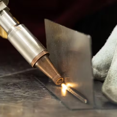
Figure 1. Laser welding.
This example demonstrates a thermo-structural simulation of a laser welding process using ANSYS. The objective is to predict:
- The transient temperature field
- The resulting thermal stresses
- The extent of the heat-affected zone (HAZ)
A simplified geometry is used to represent two plates joined by a weld as shown in Figure 2.
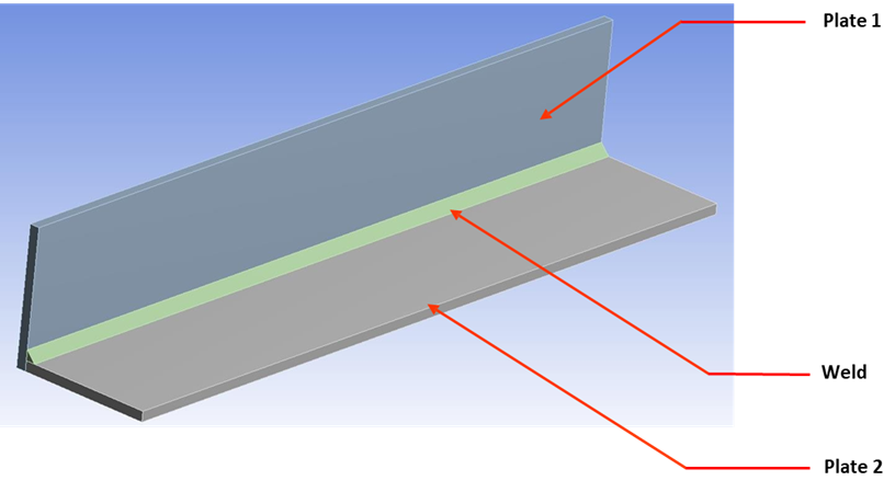
Figure 2. A simplified model.
All parts in the model are assigned the same material properties as shown below. For simplicity, no temperature dependent properties are considered. Also, material is considered to be linear elastic. Note: In physical welding, temperature-dependent properties (e.g. thermal conductivity, yield strength) are critical. Their omission here simplifies the example but limits physical accuracy.
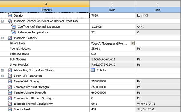
Figure 3. Material properties.
Sweep mesh is used for the three components. For the plates, three elements are defined through the thickness to capture the bending effects.
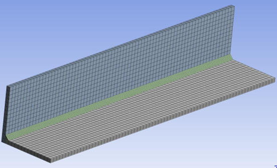
Figure 4. Mesh.
Contact Definition
Two contacts are defined:
- Plate-to-plate contact.
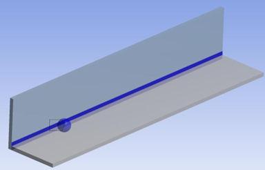
Figure 5. Contact between the plates.
- Weld-to-plate contact.
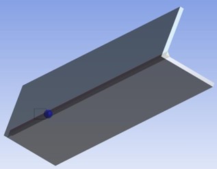
Figure 6. Contact between weld and plates (bottom view).
For the contact between weld and plates, we further define a critical Bonding temperature of 500 ºC using commands. As soon as the temperature at the contact surface (Tc) for closed contact exceeds this bonding temperature, the contact will change to “bonded”. The contact status will remain bonded for the rest of analysis, even if the temperature subsequently drops below the critical value.
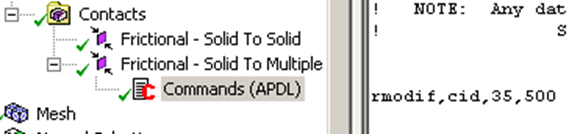
Figure 7. APDL insertion.
Install Moving Heat Source Extension
To simulate the thermal field produced by the welding process, it is necessary to model the heat source accurately. In this case, moving heat is modeled using the “Moving Heat Source Extension” ACT extension which is available for download from ANSYS support website:
https://developer.ansys.com/app/cybernet-systems-corporation/moving-heat-source-extension/4-2
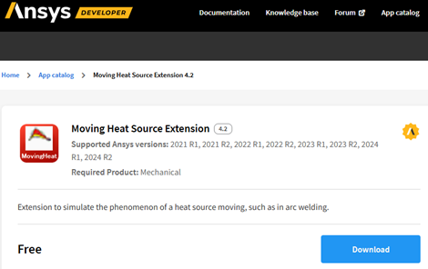
Figure 8. Moving heat source ACT extension.
Please refer to a YouTube video on how to use this extension:
https://www.youtube.com/watch?v=KuGyVu7H4gU
Moving Heat Flux
Heat source parameters:
Velocity of source=5 mm/sec
Start time=0 sec
End time of the heat source=44 sec
Intensity of laser=7.5 W/mm2
Radius of laser beam=5 mm
This represents a Gaussian-type moving heat input. The heat source is applied along a predefined path as shown in Figure 10-Figure 12.
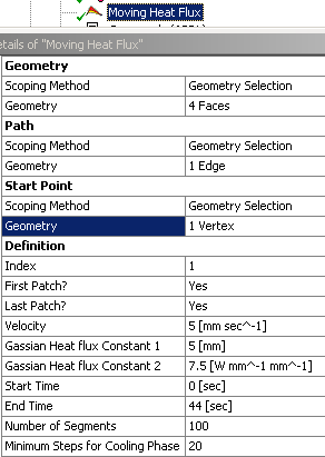
Figure 9. Details of moving heat flux.
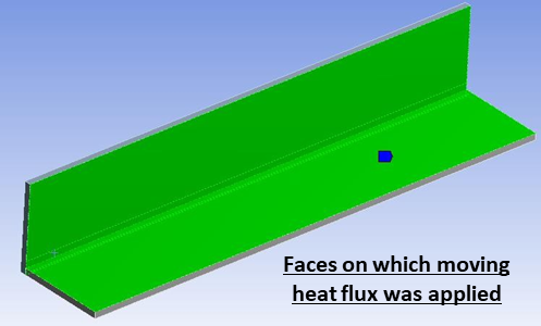
Figure 10. Geometric scope.
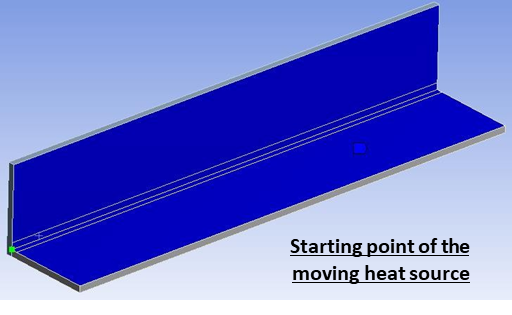
Figure 11. Start point.
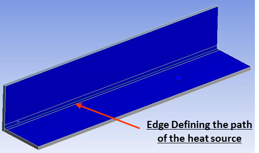
Figure 12. Path.
Convection
Convective heat loss is applied to exposed surfaces as shown in Figure 13.
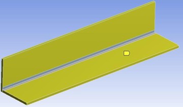
Figure 13. Geometric scope.
As shown in Figure 14, the film coefficient is temperature-dependent and is defined through tabular data (see Figure 15). This is important because heat transfer to the environment increases at higher temperatures, and constant convection coefficients can significantly underpredict cooling rates. The details of convection definition are shown in Figure 16.
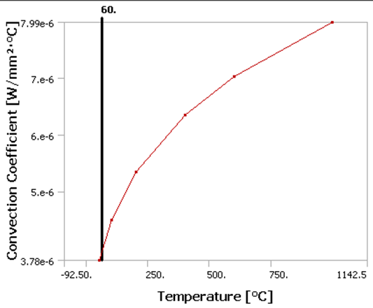
Figure 14. Convection coefficient vs. temperature.
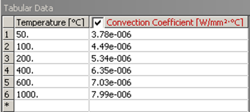
Figure 15. Tabular data for convection coefficient.
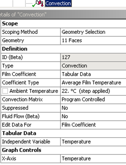
Figure 16. Details of convection.
Transient Temperature Field
The transient thermal analysis captures the evolution of the temperature field as the heat source moves. Some key observations are as follows
- Highly localized temperature peaks following the heat source
- Rapid cooling behind the heat source
- Strong thermal gradients near the weld path
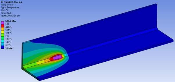
Figure 17. Temperature at 12.6 sec.
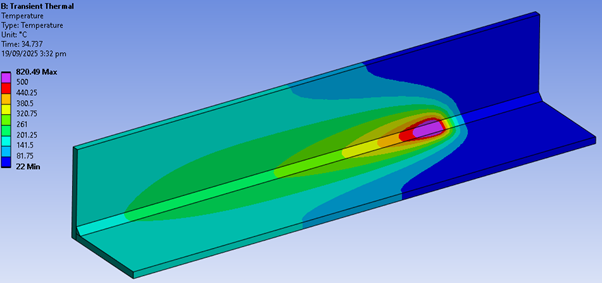
Figure 18. Temperature at 34.737 sec.
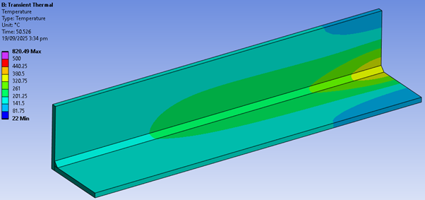
Figure 19. Temperature at 50.526 sec.
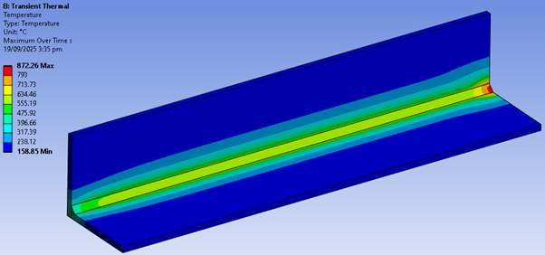
Figure 20. Maximum temperature over time.
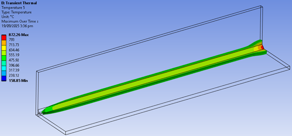
Figure 21. Heat-affected zone (the region that has seen a temperature of 500 °C or higher during the process).
Thermo-Structural Coupling
To predict stresses due to the thermal field generated by the transient thermal analysis, drag and drop a “Static Structural” module on “Transient Thermal” as shown below.
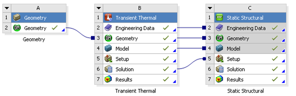
Figure 22. Project schematic.
Structural Boundary Conditions
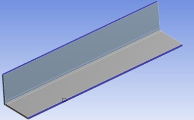
Figure 23. Frictionless support.
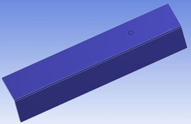
Figure 24. Compression only support (bottom and back).
Imported Temperature
Temperature from Transient thermal is then imported in the Static Structural for all the steps at which Transient thermal has written data. In total for this case there are 122 steps. Thus we define 122 steps in Static Structural and import the data at each step.
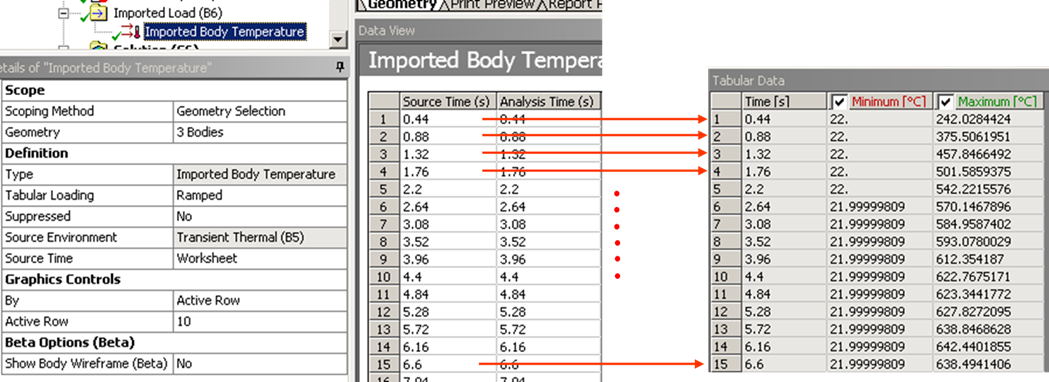
Figure 25. Import temperature load.
Stress Results
The thermal field induces significant stresses due to constrained expansion. Some key observations are as follows
- Peak stresses occur near the weld region
- Stress evolves over time as heating and cooling progress
- Residual stresses remain after cooling
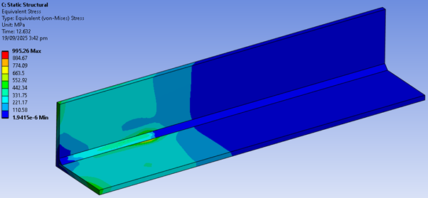
Figure 26. Von Mises stress at 12.632 sec.
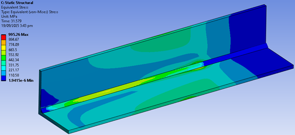
Figure 27. Von Mises stress at 31.579 sec.
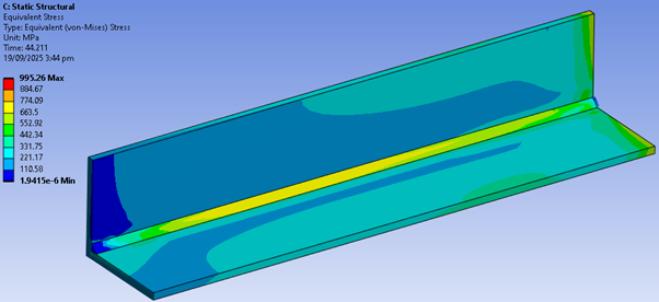
Figure 28. Von Mises stress at 44.211 sec.
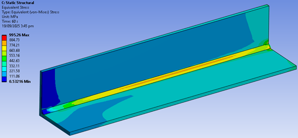
Figure 29. Von Mises stress at 60 sec.
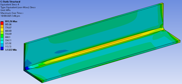
Figure 30. Maximum von Mises stress over time.
Contact Status
Contact status changes dynamically during the process:
- Initially: open or sliding contact
- As temperature increases: bonding occurs
- After bonding: interface remains permanently connected
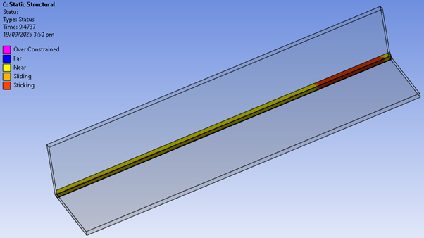
Figure 31. Contact status at 9.4737 sec (bottom view, welding starts from right to left).
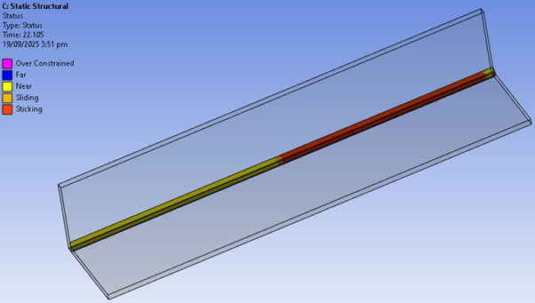
Figure 32. Contact status at 22.105 sec (bottom view, welding starts from right to left).
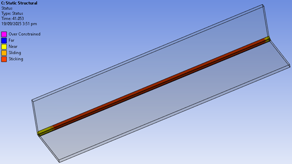
Figure 33. Contact status at 41.053 sec (bottom view, welding starts from right to left).
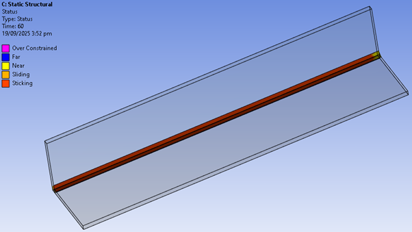
Figure 34. Contact status at 60 sec (bottom view, welding starts from right to left).
This example adopts several simplifying assumptions, including linear elastic material behaviour, temperature-independent properties, and idealized heat input, to demonstrate the workflow. While these assumptions limit physical fidelity, they provide a clear and efficient framework for understanding thermo-structural coupling in welding simulations.
