When a metal is loaded beyond its elastic limit, it no longer springs back to its original shape – it deforms permanently. Capturing this behaviour accurately in FEA requires moving beyond simple linear-elastic models and into the realm of plasticity. This post walks through the key concepts behind metal plasticity including true stress and strain, strain hardening, and hardening rules, and explains how to set up elastoplastic material models in both ANSYS and SolidWorks Simulation.

1. Engineering Stress-Strain vs. True Stress-Strain

The stress and strain quantities recorded in a standard tensile test are engineering (or nominal) values: stress is calculated using the original cross-sectional area, and strain is referenced to the original gauge length. These are convenient for small deformations, but they become increasingly inaccurate as the specimen necks and the cross-section shrinks significantly.

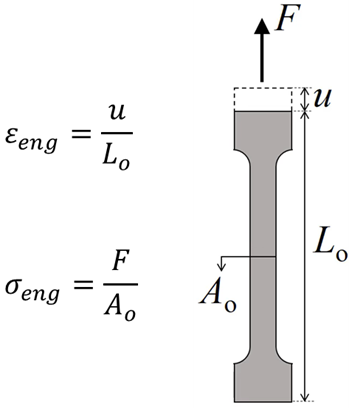
Figure 1. Engineering stress-strain.

True stress–strain, by contrast, accounts for the instantaneous geometry of the specimen at every point during the test. True stress uses the actual (current) cross-sectional area, and true strain (also called logarithmic strain) is accumulated incrementally. For large-deformation and plasticity analyses, true stress-strain must be used, as it is a more representative measure of the actual material state.

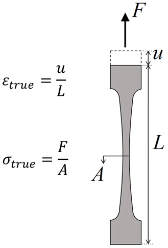
Figure 2. True stress-strain.

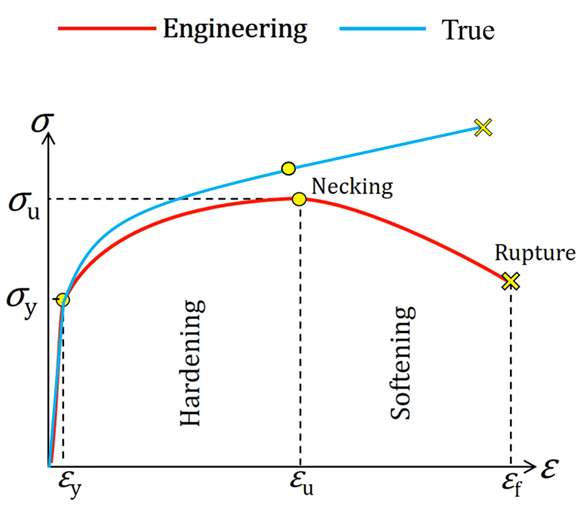
Figure 3. Engineering stress-strain vs. true stress-strain.

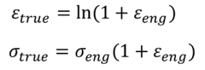
If engineering stress-strain data is available, one can convert these values to true stress-strain with the following approximations:

• After yielding, before necking:

• After necking:

• After necking (alternative method):

Extend the stress-strain curve in a straight line tangential to the necking point.

where

For most FEA applications, material data beyond the necking point is rarely needed, as structural components are not designed to operate in that regime. The pre-necking conversion formulas are therefore sufficient in the majority of practical cases.

2. Strain Hardening

When a metal is loaded beyond its yield point and then unloaded, it does not return to zero strain – a permanent plastic strain remains. If it is reloaded, it will yield again, but at a higher stress than before. This phenomenon is called strain hardening (or work hardening).

Post-yield behaviour is typically characterized as being either elastic–perfectly plastic or strain hardening behaviour, as shown in Figure 4. In the perfectly plastic case, once the stress reaches the yield point A, plastic deformation ensues, so long as the stress is maintained at Y. If the stress is reduced, elastic unloading occurs. In the hardening case, once yield occurs, the stress needs to be continually increased to drive further plastic deformation. If the stress is held constant, for example at B, no additional plastic strain accumulates, and no elastic unloading occurs either. The yield stress effectively rises with plastic strain.

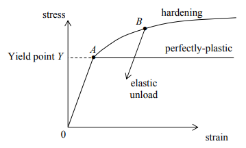
Figure 4. Uniaxial stress-strain curve (for a typical metal), showing elastic–perfectly plastic vs. strain-hardening behaviour.

The description of how the yield surface evolves with plastic deformation is called the hardening rule. The two most widely used rules are isotropic hardening and kinematic hardening.

2.1 Isotropic Hardening Rule

Isotropic hardening is where the yield surface remains the same shape but expands with increasing stress, as shown in Figure 5 and Figure 6. The yield point σ_y keeps increasing while the accumulated plastic strains are pushed further.

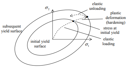
Figure 5. Isotropic hardening described in plane problems.

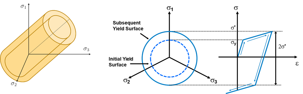
Figure 6. Isotropic hardening described in 3D principal stress state.

Note that the subsequent yield in compression is equal to the highest stress attained during the tensile phase. This means the model does not capture any asymmetry between tensile and compressive yielding introduced by prior loading.

Where to use: Isotropic hardening is often used for large strain analyses where the loading direction does not reverse. It is generally not appropriate for cyclic loading, as it cannot model the softening of yield in the reverse direction.

2.2 Kinematic Hardening Rule

To understand kinematic hardening, it helps to first understand the phenomenon it is designed to capture: the Bauschinger Effect. If a metal specimen is deformed plastically in tension up to a tensile stress of + σ_t (Figure 7) and is then subjected to a compressive strain (as indicated by the arrows in Figure 7), it will first contract elastically and then, instead of yielding plastically in compression at a stress of –σ_t as might have been expected, it is found that plastic compression starts at a lower stress (–σ_c) – a phenomenon known as the Bauschinger Effect. In simple terms: Prior plastic deformation in one direction makes yielding easier in the opposite direction.

Figure 7. Illustration of the Bauschinger Effect when the direction of straining is reversed as indicated by the arrowed dotted line [1].

The Bauschinger Effect arises because, during the initial tensile plastic straining, internal stresses accumulate in the test-piece and oppose the applied strain. When the direction of straining is reversed these internal stresses now assist the applied strain, so that plastic yielding commences at a lower stress than that operating in tension [1].

The isotropic model implies that, if the yield strengths in tension and compression are initially the same, i.e. the yield surface is symmetric about the stress axes, they remain equal as the yield surface develops with plastic strain. In order to model the Bauschinger effect where a hardening in tension will lead to a softening in a subsequent compression, one can use the kinematic hardening rule. For kinematic hardening, the yield surface remains the same shape and size but merely translates in stress space, as shown in Figure 8 and Figure 9. Subsequent yield in compression is decreased by the amount that the yield stress in tension increased, so that a 2σ_y difference between the yields (i.e.  the elastic zone) is always maintained.

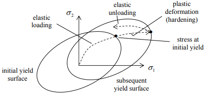
Figure 8. Kinematic hardening described in plane problems [2].

Figure 9. Kinematic hardening described in 3D principal stress state.

Depending on the stress history, one can even have the situation shown in Figure 10, where yielding occurs upon unloading, even though the stress is still tensile. However, this is physically unrealistic and reflects the main limitation of the linear kinematic hardening rule. Linear kinematic hardening may become inappropriate for very large strain because the actual Bauschinger effect evolves nonlinearly and often saturates, whereas the linear model assumes indefinite linear translation of the yield surface.

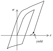
Figure 10. The limitation of linear kinematic hardening rule for very large strain simulations.

Overall, when load is monotonic, isotropic and kinematic hardening behave the same. When there is cyclic loading, isotropic hardening cannot simulate the Bauschinger effect. Therefore, when the material is expected to be under cyclic loading, kinematic hardening should be used to simulate the material. The behaviour of isotropic and kinematic hardening is not specific for von Mises yield criterion. Such behaviour is general for all yield criteria.

3. Define Plasticity in FEA

Before running a nonlinear analysis, the material’s plastic behaviour must be defined. The key decisions are:

1. Identify the yield point – the stress at which plastic deformation begins.
2. Choose perfect plasticity or hardening – perfect plasticity is conservative and simpler; hardening is more realistic.
3. If hardening: choose the hardening model – isotropic, kinematic, or combined.
4. Define the post-yield stress–strain curve using one of the following representations:

Figure 11. Perfect plasticity.

Figure 12. Bilinear hardening.

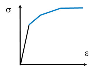
Figure 13. Multilinear hardening.

Figure 14. Nonlinear hardening.

3.1 Define Plasticity: Bilinear Hardening

Bilinear hardening is the simplest hardening model. It characterises the post-yield response with just two slopes:

1. Young’s modulus E: the tangent of the initial linear part of material engineering stress-strain curve.
2. Tangent modulus E_T : the tangent of the plastic segment of the true stress-strain curve.

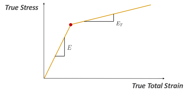
Figure 15. Define bilinear hardening.

This model is easy to calibrate from basic tensile test data and is computationally efficient, making it a good starting point when detailed stress–strain data are not available.

3.2 Define Plasticity: Multilinear Hardening in ANSYS

Multilinear hardening represents the post-yield curve as a series of straight-line segments, providing a more accurate fit to the actual material behaviour than bilinear hardening.

In ANSYS, multilinear isotropic or kinematic hardening is defined by entering a table of plastic strain vs. true stress data points. The first data point must always be (0, σ_y) – zero plastic strain at the yield stress – as shown in Figure 16. Subsequent points represent accumulated plastic strain paired with the corresponding true stress.

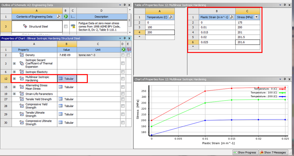
Figure 16. Define multilinear isotropic hardening in ANSYS.

Important: Do not confuse total strain with plastic strain when entering data. Plastic strain = total strain − elastic strain.

3.3 Define Plasticity: Multilinear Hardening in SolidWorks Simulation

In SolidWorks Simulation, the full stress–strain curve can be entered directly in the material library via the stress–strain data input dialog (Figure 17).

Figure 17. Stress-strain input.

Engineering strain is a small strain measure which is invalid once the strain in the model is no longer ‘small’ (approximately larger than 5%). True strain (also named logarithmic strain) should be used for large strain simulations. Depending on the analysis option and the type of material model used, different types of stress and strain that should be used as input for the stress-strain curve are summarized in the following table:

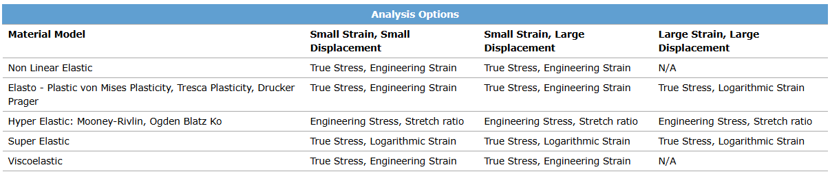
Key rules for defining the stress-strain curve in SolidWorks Simulation:

1. When defining a stress-strain curve, the first point on the curve should be the yield point of the material.
2. When a stress–strain curve is provided, material properties such as elastic modulus, yield strength, etc. will be taken from the stress-strain curve and not from the material properties table in the Material dialog box. Only the Poisson’s ratio (NUXY) will be taken from the table.
3. If the simulation requires stress states beyond the last data point entered, the software linearly extrapolates the curve using the slope defined by the last two data points. Ensure the curve extends to strains beyond the maximum expected in the analysis, or at least that the extrapolated behaviour is physically reasonable.

References

1. W. Martin, 2006. Materials for Engineering (Third Edition), Pages 37-67, https://doi.org/10.1533/9781845691608.1.37
2. Kelly, Solid Mechanics Part II: Engineering Solid Mechanics – small strain: https://pkel015.connect.amazon.auckland.ac.nz/SolidMechanicsBooks/Part_II/08_Plasticity/08_Plasticity_06_Hardening.pdf