Fatigue is one of the most important failure mechanisms in mechanical and structural engineering. A component may appear safe under a conventional static strength assessment, yet still fail after repeated loading and unloading. This is because fatigue damage accumulates gradually over time, often under stress levels much lower than the material’s static strength limit.
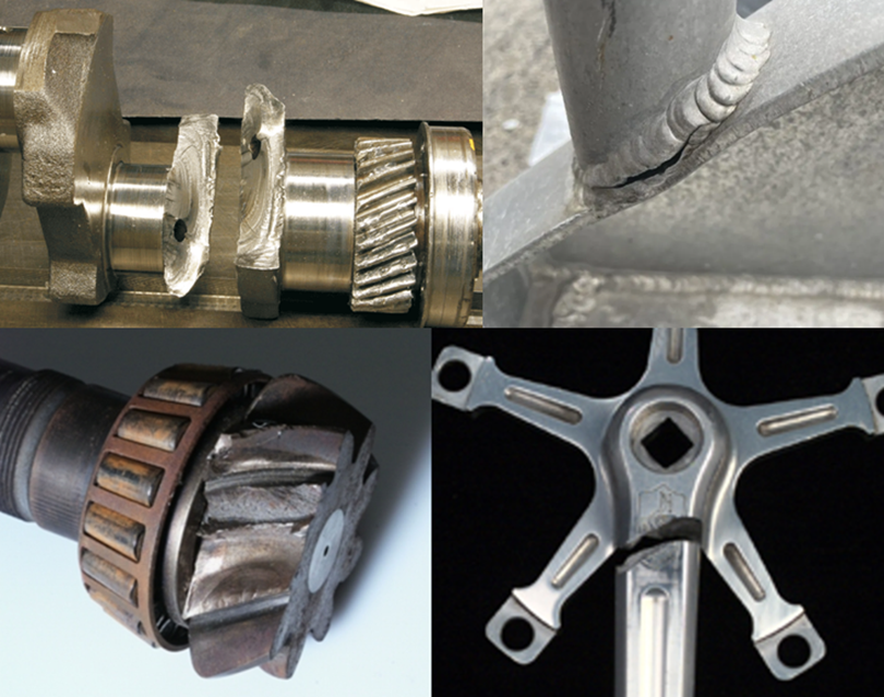
Figure 1. Examples of fatigue failure.
Conventional linear or nonlinear structural analysis can predict deformation, stress, strain, and safety margins under a given set of loads and restraints. However, these analyses do not automatically predict fatigue failure. A fatigue assessment is therefore needed when a component is expected to experience repeated cyclic loading during service.
This article introduces the basic concepts of fatigue analysis, with a focus on the stress-life approach commonly used for high-cycle fatigue. It also explains how fatigue analysis is implemented in Ansys Mechanical, with particular emphasis on mean stress correction.
1. What Is Fatigue?
Fatigue refers to the progressive weakening of a material or component under repeated loading. The key point is that fatigue failure can occur even when the applied stress is below the static allowable stress.
A typical fatigue failure process includes three stages:
- Crack initiation
Small cracks begin to form, often at microscopic imperfections, surface scratches, weld toes, sharp corners, holes, notches, or other stress concentrators. - Crack propagation
Once initiated, the crack grows gradually under continued cyclic loading. - Final fracture
As the crack grows, the remaining intact section becomes too weak to carry the load. Sudden final failure then occurs.
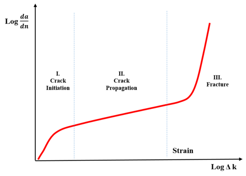
Figure 2. Stages of failure due to fatigue.
Fatigue cracks often initiate at the surface because the surface is exposed to environmental effects and frequently contains the highest local stress. This is why surface finish, surface treatment, residual stress, corrosion protection, and manufacturing quality can strongly influence fatigue life.
2. High-Cycle and Low-Cycle Fatigue
Fatigue is commonly divided into two broad categories.
High-cycle fatigue
High-cycle fatigue refers to cases where the number of load cycles before failure is relatively large, often in the range of 1e4 to 1e9 cycles. The stress level is usually low enough that the material response remains mostly elastic. For high-cycle fatigue, the stress-life method, also known as the S-N method, is commonly used.
Low-cycle fatigue
Low-cycle fatigue occurs when the number of cycles to failure is relatively small. The stress level is usually high enough to cause plastic deformation. In this case, fatigue behaviour is better described using a strain-life approach.
In many practical engineering applications, especially when the component remains largely elastic, the stress-life method provides a useful and efficient fatigue assessment approach.
3. Constant Amplitude and Variable Amplitude Loading
Fatigue loading can be classified according to how the load varies with time.
Constant amplitude loading
In constant amplitude loading, the maximum and minimum stress levels remain constant from cycle to cycle. This is the simplest fatigue loading case and is commonly used for introductory fatigue analysis.
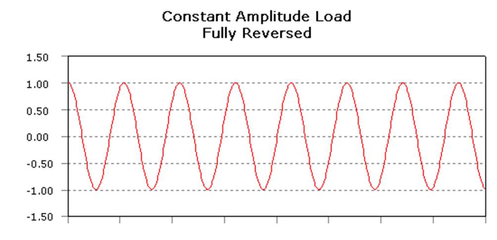
Figure 3. Constant amplitude loading.
Variable amplitude loading
In variable amplitude loading, the stress history changes over time. Real-world loading is often variable amplitude, such as road loading, wind loading, wave loading, vibration loading, or machine operation under changing service conditions.
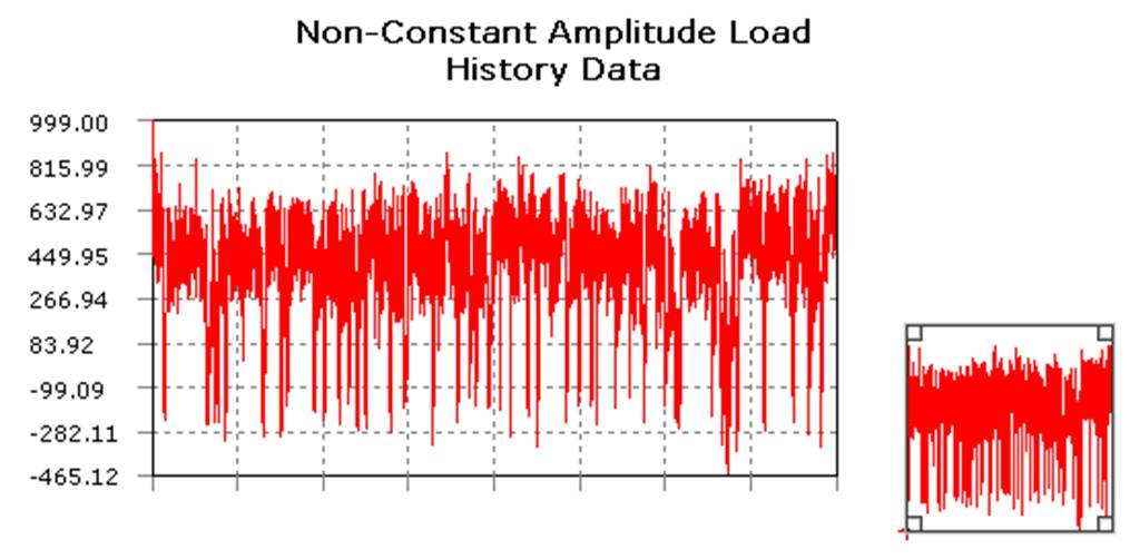
Figure 4. Variable amplitude loading.
Variable amplitude fatigue usually requires additional treatment, such as load history input, cycle counting, and cumulative damage models.
4. Proportional and Non-Proportional Loading
Another important distinction is between proportional and non-proportional loading.
Proportional loading
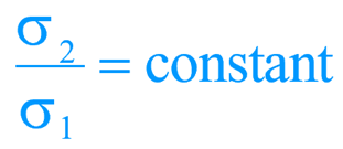
In proportional loading, the ratio between principal stresses remains constant and the principal stress directions do not change with time. This means that the stress state scales up or down in a consistent way during the loading cycle.
Non-proportional loading
In non-proportional loading, the relationship between stress components changes with time. Examples include:
- alternating between different load cases;
- an alternating load combined with a static load;
- nonlinear contact or nonlinear boundary conditions;
- changing principal stress directions.
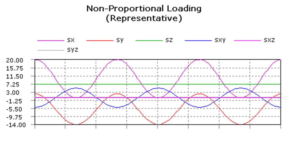
Figure 5. Non-proportional loading.
Non-proportional fatigue is more complex because a single scalar stress history may not fully describe the fatigue-driving stress state.
5. Basic Stress Definitions in Fatigue
For constant amplitude fatigue loading, several stress quantities are commonly used.
Let the maximum and minimum stresses in a cycle be:

and

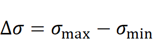
The stress range is:
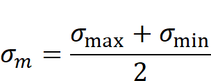
The mean stress is:
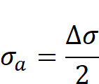
The stress amplitude, also called the alternating stress, is:
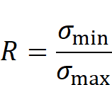
The stress ratio is:
Two common special cases are:
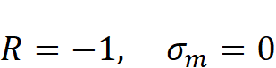
- Fully reversed loading:
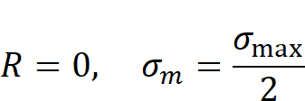
- Zero-based loading:
These definitions are essential because fatigue life depends not only on the stress amplitude, but also on the mean stress.
6. The Stress-Life S-N Approach
The stress-life approach is based on the relationship between stress amplitude and the number of cycles to failure. This relationship is represented by an S-N curve, where:
- S represents stress amplitude;
- N represents the number of cycles to failure.
In general, a higher stress amplitude leads to a shorter fatigue life, while a lower stress amplitude leads to a longer fatigue life.
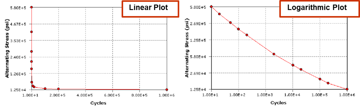
Figure 6. Example S-N curves (the same data is shown here with both a linear and logarithmic plot).
S-N curves are usually obtained experimentally by testing specimens under cyclic loading. Because fatigue data often spans several orders of magnitude in life, S-N curves are commonly plotted on logarithmic axes.
7. Fatigue Strength and Endurance Limit
Two important terms are commonly used when interpreting S-N curves.
Fatigue strength
Fatigue strength is the stress amplitude that causes failure at a specified number of cycles. For example, if a material fails at 1e6 cycles under a certain alternating stress, that stress may be referred to as the fatigue strength at 1e6 cycles.
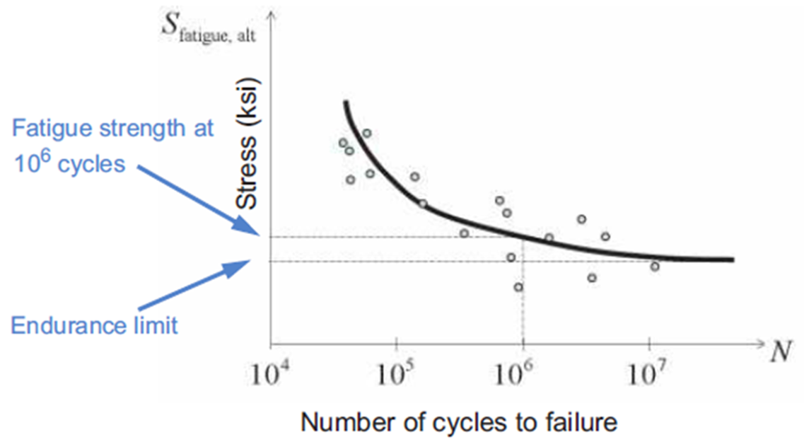
Figure 7. Fatigue strength and endurance limit.
Endurance limit
The endurance limit, also called the fatigue limit, is the highest alternating stress below which the material can theoretically sustain an infinite number of cycles without fatigue failure. In practice, the endurance limit is usually defined for fully reversed loading. Not all materials exhibit a clear endurance limit. Many steels do, whereas aluminium alloys and some other materials often show a continuously decreasing S-N curve.
8. Why Mean Stress Matters
Mean stress is one of the most important factors in fatigue analysis. For the same stress amplitude, fatigue life can change significantly depending on whether the mean stress is tensile, zero, or compressive.
A useful practical interpretation is:
- Tensile mean stress is harmful.
It tends to open cracks and accelerate crack growth, reducing fatigue life. - Compressive mean stress is usually beneficial.
It tends to suppress crack opening and can increase fatigue life. - Zero mean stress is the standard reference case for many S-N curves.
Many fatigue tests are performed under fully reversed loading, where R=-1 and .
This creates a practical problem. If the available S-N curve is based on fully reversed loading, but the actual component experiences a non-zero mean stress, the S-N curve cannot be used directly without adjustment.
This is where mean stress correction becomes important.
9. Mean Stress Correction
Mean stress correction is used to account for the effect of non-zero mean stress when only limited fatigue data are available. In an ideal situation, fatigue test data would be available for multiple mean stress levels or multiple stress ratios. If such data are available, they should generally be used directly. In Ansys Mechanical, this corresponds to using Mean Stress Curves.
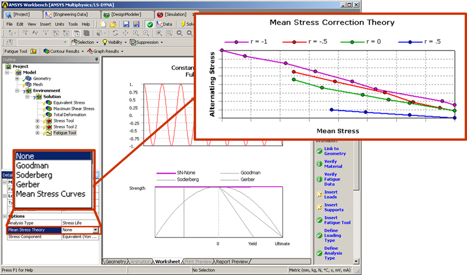
Figure 8. Using Mean Stress Curves in Fatigue Tool.
However, in many practical cases, only one S-N curve is available, often for fully reversed loading. In that situation, a mean stress correction theory can be used to modify the fatigue assessment.
The basic idea is:
- for a fixed fatigue life, increasing tensile mean stress reduces the allowable stress amplitude;
- as the stress amplitude approaches zero, the allowable mean stress approaches a material strength limit;
- compressive mean stress may improve fatigue life, although some correction methods conservatively ignore this benefit.
Ansys Mechanical provides common mean stress correction options (as shown in Figure 8), including:
- None
- Mean Stress Curves
- Goodman
- Soderberg
- Gerber
10. Common Mean Stress Correction Theories
10.1 No mean stress correction
If None is selected, the fatigue calculation ignores mean stress effects. This may be acceptable only when the mean stress is negligible or when the S-N data already corresponds closely to the actual loading condition. If the component has significant tensile mean stress, ignoring mean stress may produce unconservative fatigue life predictions.
10.2 Mean Stress Curves
The most reliable approach is to use experimentally measured S-N curves at different mean stress levels or stress ratios. This avoids relying on an approximate correction theory. If sufficient fatigue data are available, Mean Stress Curves are preferable to theoretical correction models.
However, such data are not always available.
10.3 Goodman correction
The Goodman correction is widely used and is often considered suitable for relatively low-ductility metals. It is based on a linear relationship between stress amplitude and tensile mean stress.
A common form is:
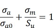
where:
- is the allowable stress amplitude under non-zero mean stress;
- is the allowable stress amplitude under fully reversed loading;
- is the mean stress;
- is the ultimate tensile strength.
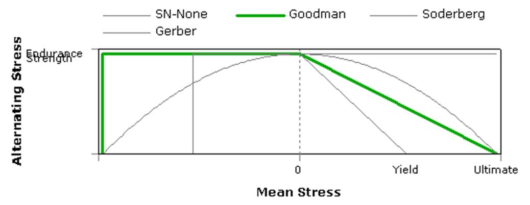
Figure 9. Goodman correction.
The Goodman model reduces allowable alternating stress as tensile mean stress increases. In many implementations, no beneficial correction is applied for compressive mean stress, which is a conservative assumption.
10.4 Soderberg correction
The Soderberg correction is generally more conservative than Goodman because it uses yield strength instead of ultimate tensile strength.
A common form is:
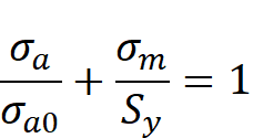
where is the yield strength.
Because is normally lower than , the Soderberg correction predicts a lower allowable alternating stress for the same tensile mean stress. It is therefore more conservative.
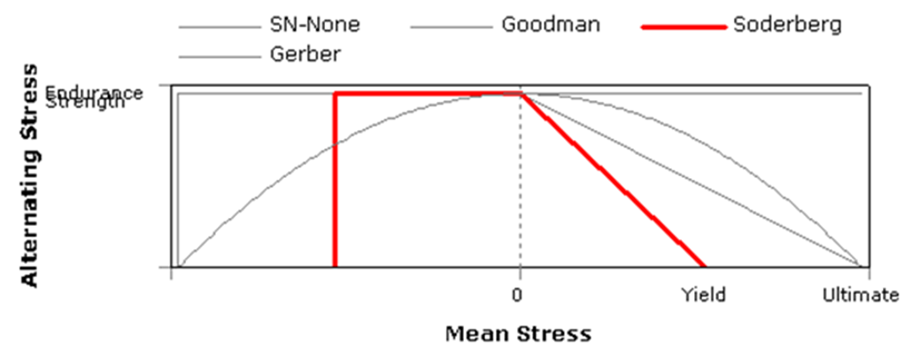
Figure 10. Soderberg correction.
This method may be used when a conservative design assessment is desired, but it can be overly conservative for some ductile metals.
10.5 Gerber correction
The Gerber correction is a parabolic mean stress correction model. It is often considered more suitable for ductile metals under tensile mean stress.
A common form is:
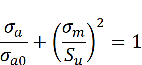
Compared with Goodman and Soderberg, Gerber is usually less conservative for tensile mean stress in ductile materials.
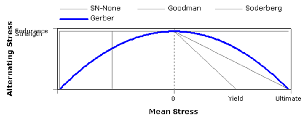
Figure 11. Gerber correction.
However, one limitation is that the Gerber curve may predict an undesirable effect under compressive mean stress in some cases. Therefore, its use should be considered carefully, especially if compressive mean stress is significant.
11. Practical Guidance on Mean Stress Correction
A practical selection strategy is as follows:
- Use measured mean stress S-N curves if available.
This is usually the best option because it is based directly on experimental data. - Use Goodman for a general conservative engineering estimate.
Goodman is widely used and relatively simple. - Use Soderberg when a more conservative estimate is required.
This may be appropriate when yield-related limitations are important or when design conservatism is required. - Use Gerber for ductile metals when a less conservative tensile mean stress correction is justified.
This should be supported by engineering judgement and material behaviour. - Do not ignore mean stress if the loading is not fully reversed.
For zero-based loading or tensile-biased cyclic loading, mean stress can significantly reduce predicted fatigue life.
A particularly important point is that a zero-based load is not equivalent to a fully reversed load. Even if the stress range appears moderate, zero-based loading has a positive mean stress, which can reduce fatigue life compared with fully reversed loading.
12. Fatigue Material Properties in Ansys Mechanical
To perform a stress-life fatigue analysis in Ansys Mechanical, fatigue material data must be defined. The most important input is the S-N curve.
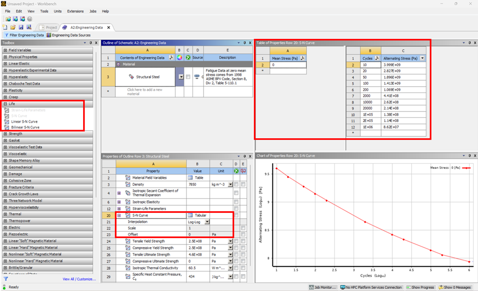
Figure 12. Defining S-N curve in Engineering Data.
The S-N curve defines the relationship between alternating stress and cycles to failure. Depending on the available material data, the curve may be defined using different interpolation methods:
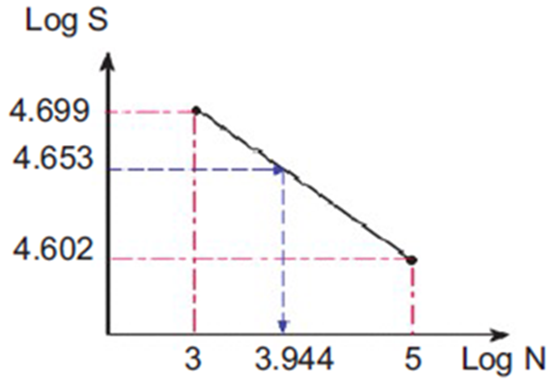
- Log-log interpolation
Suitable when both stress and life vary over wide ranges and only limited data points are available.
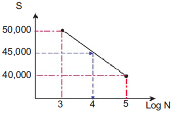
- Semi-log interpolation
Suitable when the stress range is relatively small compared with the variation in fatigue life.
- Linear interpolation
Suitable when many data points are available and the data spacing supports linear interpolation.
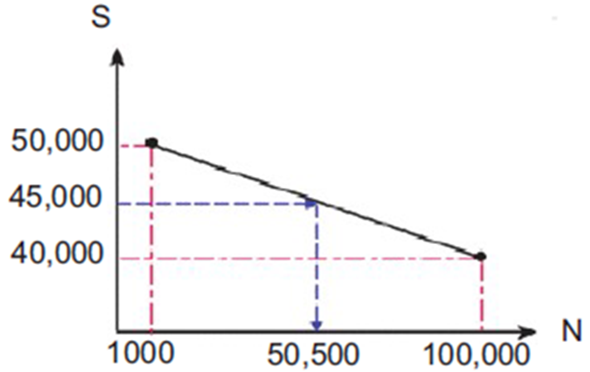
The selected interpolation method can influence the calculated fatigue life, especially when the stress falls between sparse data points.
13. Loading Type in the Ansys Fatigue Tool
After inserting a Fatigue Tool in Ansys Mechanical, the loading type must be specified. Common options include:
- Fully Reversed
- Zero-Based
- Ratio
- History Data
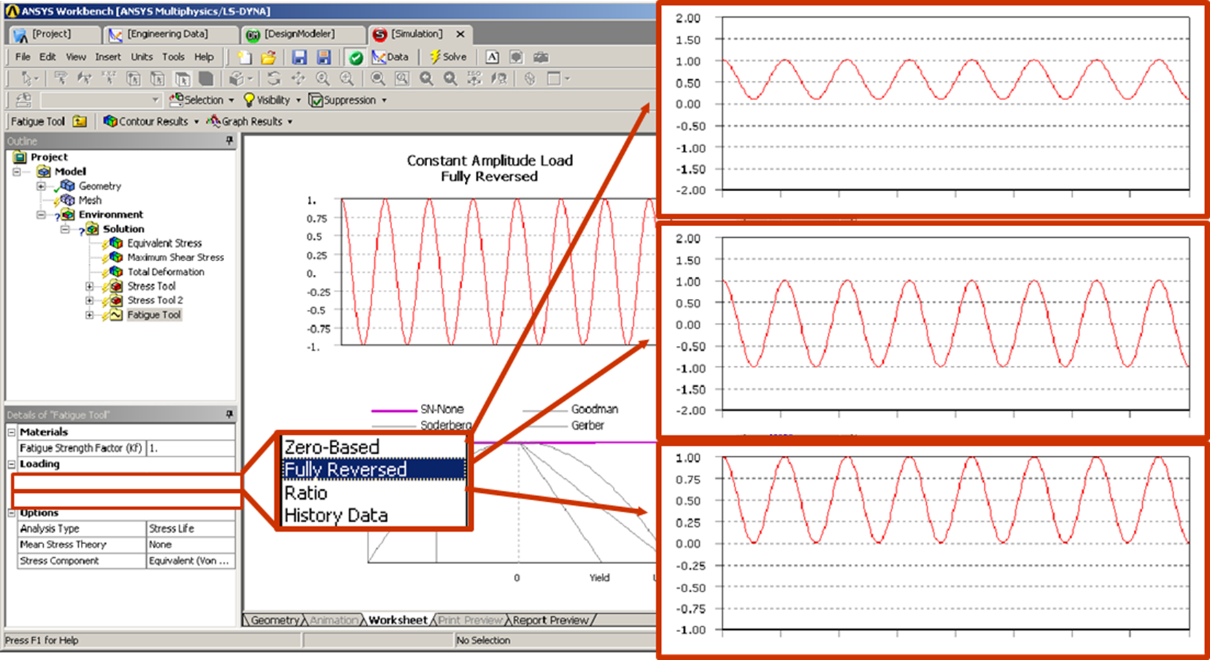
Figure 13. Loading types.
For constant amplitude fatigue:
- Fully Reversed corresponds to R=-1;
- Zero-Based corresponds to R=0;
- Ratio allows the user to define a specific stress ratio.
The loading type determines the relationship between the minimum and maximum stress in the fatigue cycle. Therefore, it directly affects the stress amplitude and mean stress used in the fatigue calculation.
14. Fatigue Strength Reduction Factor
In real components, fatigue performance may differ from ideal laboratory specimens. This difference may be caused by:
- surface finish;
- size effects;
- manufacturing defects;
- residual stresses;
- welds;
- notches;
- environmental effects;
- material processing.
In Ansys Mechanical, these effects can be represented using a fatigue strength reduction factor.
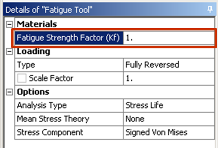
Figure 14. Fatigue strength reduction factor.
This factor modifies the alternating stress used in the fatigue calculation. A value less than 1 reduces the effective fatigue strength of the component compared with the test specimen. This is important because fatigue test specimens are often polished, carefully manufactured, and tested under controlled conditions. Real components are usually less ideal.
15. Stress Component Selection
Fatigue test data are often obtained from uniaxial fatigue specimens. However, a real component usually experiences a multiaxial stress state. Therefore, Ansys Mechanical needs to convert the local stress tensor into a scalar stress quantity that can be compared with the S-N curve.
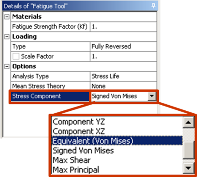
Figure 15. Defining Stress Component in Fatigue Tool.
The Stress Component setting controls this conversion. Possible choices include:
- individual normal stress components;
- individual shear stress components;
- maximum principal stress;
- maximum shear stress;
- equivalent von Mises stress;
- signed equivalent stress.
The selected stress component can significantly affect fatigue life. For example:
- maximum principal stress may be appropriate when fatigue cracking is controlled by tensile opening;
- equivalent von Mises stress may be appropriate for ductile metals under multiaxial loading;
- shear stress may be relevant when fatigue is torsion or shear dominated;
- signed equivalent stress can help preserve the effect of tensile or compressive mean stress.
The choice should be based on material behaviour, expected failure mechanism, fatigue data, and the local stress state.
16. Biaxiality Indication
Biaxiality indication is a useful diagnostic result in Ansys Mechanical. It helps determine whether the local stress state is similar to the stress state used to generate the fatigue data. The biaxiality indication is based on the ratio between principal stresses, with the principal stress closest to zero ignored.
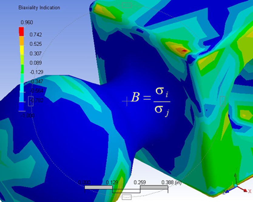
Figure 16. Biaxiality indication plot.
Typical interpretations are:
- 0: uniaxial stress state;
- -1: pure shear state;
- 1: biaxial stress state.
This result is especially useful at the critical fatigue location. If the fatigue data are based on uniaxial testing but the critical location is strongly shear-dominated or biaxial, the fatigue prediction should be interpreted carefully. Biaxiality indication does not directly calculate fatigue life. Instead, it helps assess whether the selected fatigue method and stress component are physically appropriate.
17. Reviewing Fatigue Results
Several fatigue results are commonly reviewed in Ansys Mechanical.
Life
Fatigue life shows the predicted number of cycles to failure. If the alternating stress is below the lowest stress defined in the S-N curve, Ansys may report the maximum life associated with the S-N curve data.
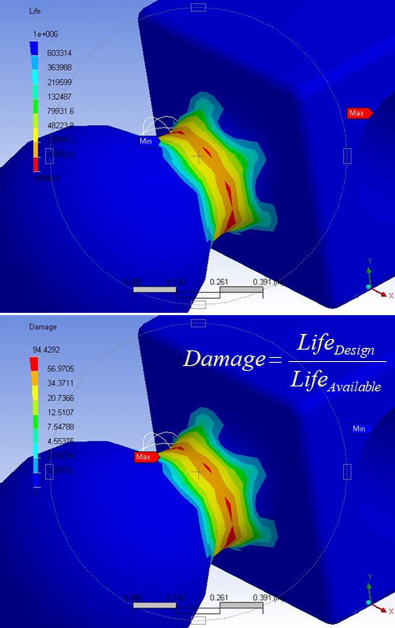
Figure 17. Life and damage plots.
Damage
Damage is usually defined as:

If damage is greater than 1, the component does not meet the specified design life.
Safety factor
The fatigue safety factor indicates how much the stress could be scaled before the component reaches the specified design life. A fatigue safety factor greater than 1 indicates that the component is predicted to survive the design life under the given loading assumptions.
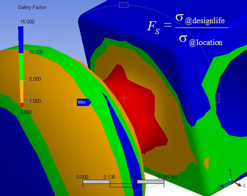
Figure 18. Safety factor plot.
Equivalent alternating stress
Equivalent alternating stress is the stress used to query the S-N curve after accounting for the loading type, mean stress treatment, and selected stress component. This is one of the most important fatigue result quantities because it directly links the FEA stress result to the fatigue material data.
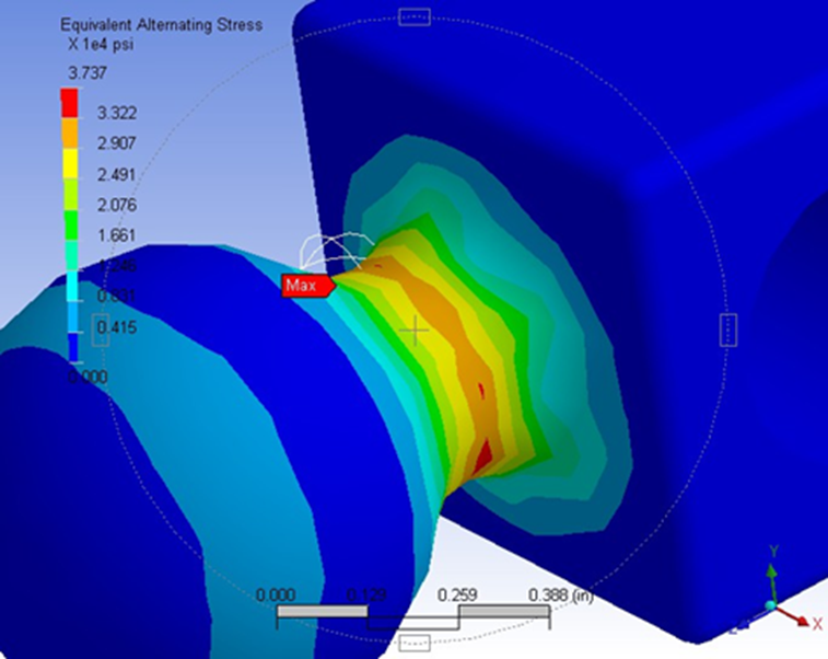
Figure 19. Equivalent alternating stress plot.
Fatigue sensitivity
Fatigue sensitivity shows how fatigue life, damage, or safety factor changes as the load is varied. This can help identify whether fatigue performance is highly sensitive to small changes in loading.
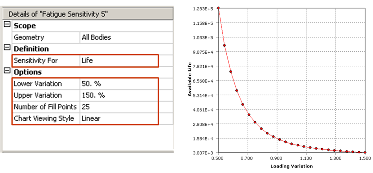
Figure 20. Fatigue sensitivity plot.
18. Recommended Workflow for Stress-Life Fatigue Analysis
A typical stress-life fatigue workflow in Ansys Mechanical is:
- Define fatigue material properties, including the S-N curve.
- Set up and solve the structural analysis.
- Insert the Fatigue Tool.
- Specify the loading type.
- Select the treatment of mean stress effects.
- Choose an appropriate stress component.
- Define any fatigue strength reduction factor if needed.
- Solve and review fatigue results.
- Check life, damage, safety factor, equivalent alternating stress, and biaxiality indication.
- Reassess assumptions if the critical location has a strongly multiaxial or shear-dominated stress state.
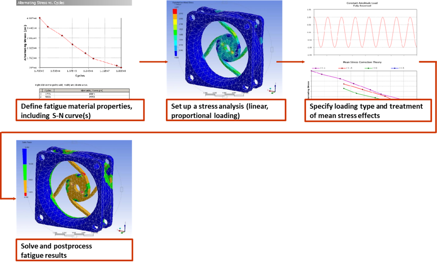
Figure 21. A typical stress-life fatigue workflow in Ansys Mechanical.
19. Key Takeaways
Fatigue failure is caused by repeated loading and can occur even when stresses are below the static strength limit. For high-cycle fatigue, the stress-life method provides a practical way to estimate fatigue life using S-N curves.
However, fatigue life depends on more than stress amplitude alone. Mean stress, surface condition, geometry, residual stress, environment, material processing, and multiaxial stress state can all influence fatigue behaviour.
Among these factors, mean stress correction is particularly important. Tensile mean stress usually reduces fatigue life, while compressive mean stress may improve it. If multiple S-N curves at different mean stresses are available, they should generally be used. If not, correction theories such as Goodman, Soderberg, or Gerber provide approximate ways to account for mean stress effects.
In Ansys Mechanical, a reliable fatigue assessment requires more than simply inserting a Fatigue Tool. The user must carefully define the S-N data, loading type, mean stress treatment, stress component, and fatigue strength correction factors. Results such as equivalent alternating stress and biaxiality indication should then be reviewed to ensure that the fatigue assumptions are physically reasonable.
Fatigue analysis is therefore not just a post-processing step. It is an engineering judgement process that connects material testing, stress analysis, loading conditions, and failure mechanisms.

